Regularization of seismic inversions for acoustic impedance models

Adam Allan

My project is a study of the regularization of seismic inversions for acoustic impedance models from synthetic seismic data. In particular, I have studied the applicability of the Gaussian hyperprior regularization method from image processing presented by Calvetti and Somersalo (2007). Seismic data is inherently band-limited, insufficient, noise-corrupted, and incomplete; as a result, solutions from their inversions can be unstable, ill-defined, and infinite in number. In order to overcome these issues, a priori information about the desired model solution is introduced to the inversion to induce stability and constrain the solutions to geologically-possible models.

The synthetic seismograms were created from a lithologic model loosely based on the Williston Basin, North Dakota. A 180-time sample acoustic impedance (AI) model was generated from velocity and porosity values from Sheriff and Geldart (1982) with a sampling interval of 7.143 ms. These AI values were used to compute a reflectivity series that could be convolved with a Ricker wavelet to generate synthetic seismograms. Note, the wavelet had a peak frequency of 30 Hz and 7.143 ms sampling interval. The seismogram is then made into 2 separate data sets by the addition of 5% and 10% Gaussian white noise and run through conjugate gradient least squares, Tikhonov regularization, total variation regularization, and Gaussian hyperprior regularization algortihms to generate AI model solutions.

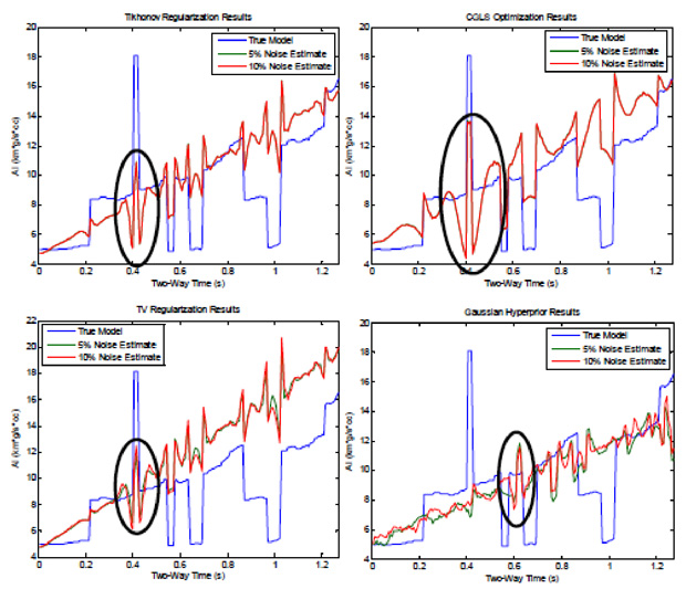
The standard deviation and frequency spectrum of each solution’s difference series, difference of true model and model solution at each time value, were computed in order to quantify the ability of each method to reproduce the sharp discontinuities present in AI models. As can be seen in the attached figure, the Tikhonov, CGLS, and total variation solutions exhibit extensive smoothing of the encircled sharp discontinutiy. The frequency spectra of these solutions identified that the error in the difference series was derived from frequencies outwith the pass-band of the Ricker wavelet used in the generation of the seismograms. The lacking high frequencies prevent the reproduction of sharp discontinuities, since infinitely many frequencies are required to reproduce a perfectly orthogonal discontinuity; while the missing low frequencies prevent the reproduction of exact AI magnitudes. The Gaussian hyperprior solution clearly shows improved reproduction of the discontinuity; however, there is a ~0.2 second time stretch in the solution due to a bug in the regularization code. Subsequently, additional work must be conducted to generate a better reproduction of the true model; however, the desired result, i.e. better representation of the discontinuities, is achieved, and, as a result, the method shows great promise.

Honors Advisor:
Dr. Mrinal K Sen