Methodology
Sample Preparation
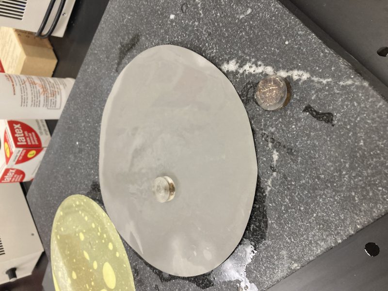
I collected whole individual garnets in the field at the outcrop in Bulgaria. I wanted to use an individual garnet instead of one in a thin section to ensure that I was analyzing the true middle of the grain. I mounted the best garnet in epoxy, cut the grain directly down the middle, and polished the surface using a series of fine grit sandpapers.
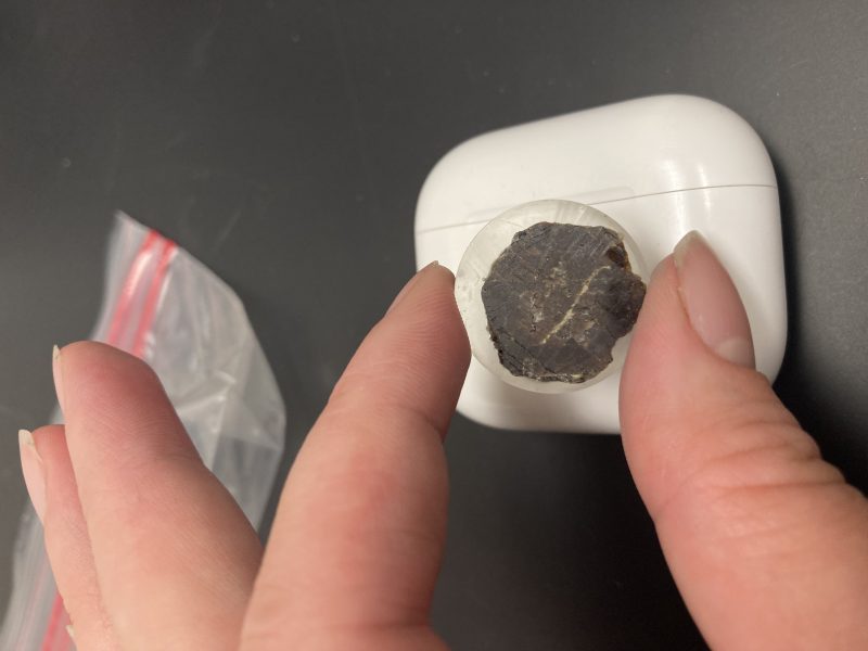
Polishing my garnet.
Final polished garnet half.
Standards and Analyte Selection
I selected the NIST610, NIST612, and BVHO external standards to use as these have been previously applied to LA-ICP-MS garnet mapping with success (e.g., Woodhead et al., 2007; Raimondo et al., 2017). I used 24Si as my internal standard. The unknowns were assigned a value of 17.6673 wt% obtained from averaging 8 representative microprobe analyses of garnet obtained from the same unit by Petrik et al. (2016). I analyzed 11 elements for both my transects and maps: 140Ce, 232Th, 90Zr, 89Y, 153Eu, 172Yb, 175Lu, 238U, 47Ti, 52Cr, and 137Ba
Instrument Tuning
I began by warming up the instruments and conducting a final x-y-z check on the sample positions. Then, the instrument was tuned up in solution mode before being switched to laser mode.
| Tuning Parameters for Solution Mode ICP-MS | |
| Plasma Conditions | |
| RF Power (W) | 1600 |
| RF Matching (V) | 1.7 |
| Sample Depth (mm) | 8 |
| Torch-H (mm) | 0.2 |
| Torch-V (mm) | -0.2 |
| Carrier Gas (L/min) | 0.88 |
| Makeup Gas (L/min) | 0.33 |
| Nebulizer Pump (rps) | 0.1 |
| S/C Temp (℃) | 2 |
| Ion Lenses | |
| Extract 1 (V) | 3 |
| Extract 2 (V) | -155 |
| Omega Bias-ce (V) | -22 |
| Omega Lens-ce (V) | 2.2 |
| Cell Entrance (V) | -30 |
| QP Focus (V) | 2 |
| Cell Exit (V) | -50 |
| Octopole Parameters | |
| OctP RF (V) | 190 |
| OctP Bias (V) | -6 |
| Q-Pole Parameters | |
| AMU Gain | 126 |
| AMU Offset | 128 |
| Axis Gain | 0.9999 |
| Axis Offset | 0 |
| QP Bias (V) | -3 |
| Detector Parameters | |
| Discriminator (mV) | 8 |
| Analog HV (V) | 1750 |
| Pulse HV (V) | 1360 |
Tuning parameters for LA-ICP-MS:
| Variables/Parameters | LA-ICP-MS Tuning |
| Laser energy (%) | 75 |
| Fluence variation (J/cm2) | 3.65 |
| Rep Rate (Hz) | 10 |
| Spot (μm) | 75 |
| Scan rate (μm/s) | 5 |
| He (mL/min) | 800 |
| Ar (mL/min) | 750 |
| Sampling Depth (mm) | 6 |
| Tuning Standard | NIST612 |
| 141Pr (ppm) | 37.2 |
| 141Pr (cps) | 3993.4 |
| 141Pr (cps/ppm) | 1073.4 |
| 248/232 (% oxide production) | 0.262 |
| 238/232 (% fractionation) | 131.095 |
Tests on Representative Unknowns
For my tests on representative unknows, I calculated the fluence (J/cm2) at different laser energies (%) in order to optimize laser conditions.
| Laser Energy (%) | Fluence (J/cm2) |
| 45 | 2.0 |
| 50 | 2.3 |
| 55 | 2.5 |
| 60 | 2.7 |
| 65 | 3.0 |
| 70 | 3.3 |
| 75 | 3.7 |
| 80 | 4.0 |
| 85 | 4.4 |
| 90 | 4.7 |
| 95 | 5.0 |
| 100 | 5.4 |
After I figured out the fluence at the different energies, I ran tests at 65, 75, 85, and 95% energies to select the optimal laser energy for pre-ablation and ablation. I was looking for the laser energy that was closest to ~4 J/cm2.
| Laser Energy (%) | Fluence (J/sec2) |
| 65 | 3.0 |
| 75 | 3.7 |
| 85 | 4.4 |
| 95 | 4.74 |
The testing showed that a laser energy between 75% and 85% is the closest to ~4 J/cm2, so I set my laser energy to 80% for pre-ablation and ablation.
To calculate integration times for line scans, I used a 0.020 ms analysis time for 12 analytes. This calculation, 12*0.020 = 0.24 s, gave me the sum of all mass integration time (s). The sampling period was 0.2672 s, which yielded a measurement time = 89.82%.
The calculations for the estimate of the total analysis time for maps are shown in the two tables below:
| 10×10 µm Map | |
| Number of Analytes | 12 |
| Int (s) | 0.02 |
| Sum Int | 0.24 |
| Total Int (89.82036% measurement time) | 0.2672 |
| Scan Rate (µm/s) | 41 |
| Map Area (µm x µm) | 1000 x 1000 |
| Time of 1 Vertical Line (s) | 24.39024 |
| Gas Blank Time (s) | 3 |
| Total Time per Line | 27.39024 |
| No. of Vertical Lines | 100 |
| Time for Map (min) | 45.65041 |
| 25×25 µm Map | |
| Number of Analytes | 12 |
| Int (s) | 0.05 |
| Sum Int | 0.6 |
| Total Int (95.66327% measurement time) | 0.6272 |
| Scan Rate (µm/s) | 41 |
| Map Area (µm x µm) | 1000 x 1000 |
| Time of 1 Vertical Line (s) | 24.39024 |
| Gas Blank Time (s) | 3 |
| Total Time per Line | 27.39024 |
| No. of Vertical Lines | 40 |
| Time for Map (min) | 18.26016 |
Pre-ablation and Ablation Parameters
I pre-ablated both the standards and samples to remove contaminates and smooth out the surface for analysis. The parameters we used for pre-ablation and ablation are shown below:
| Variables/Parameters | Pre-Ablation Parameters | Line scan Ablation Parameters | Map Ablation Parameters |
| Laser energy (%) | 75 | 80 | 80 |
| Fluence variation (J/cm2) | 3.2 | 3.72 | 3.74 |
| Rep Rate (Hz) | 10 | 10 | 20 |
| Spot (μm) | 125×125 | 40×100 | 25×25/10×10 |
| Scan rate (μm/s) | 100 | 15 | 41 |
| He (mL/min) | 850 | 800 | 800 |
| Ar (mL/min) | 750 | 250 | 750 |
| Sampling Depth (mm) | n/a | 6 | 6 |
| Gas Blank (s) | n/a | 60 | 60 |
I made two sets of maps of the same 1mmx1mm area along one of my line scans. The ablation parameters for each set of maps are identical except for spot size. I chose to vary spot size between the two maps to see how much more data can be obtained with a smaller spot size, which takes significantly longer to analyze than a larger spot size. The 25×25 μm map took about 30 minutes to analyze, whereas the 10×10 μm map took about an hour and a half (both times were longer than estimated).
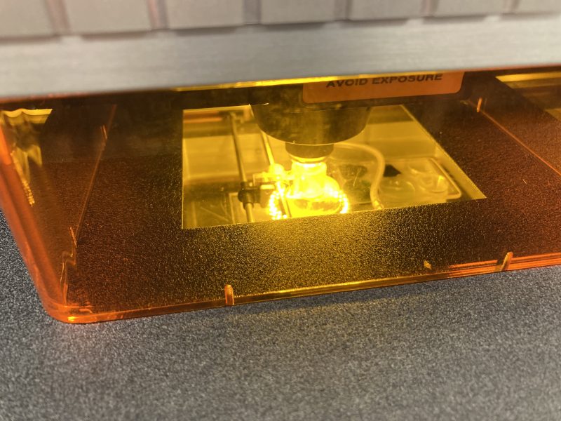
Pre-ablation of my garnet.
Data Collection
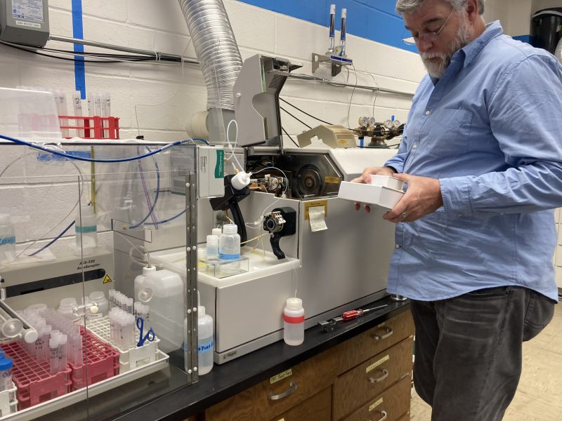
The data was collected with a New Wave Research UP193-FX fast excimer (193 nm wavelength, 4–6 ns pulse width) laser system on the Agilent 7500ce LA-ICP-MS in Dr. Nate Miller’s lab (with a great deal of his help) at the University of Texas Austin. Before developing my final method, running tests on unknowns, and the actual analysis, I selected my transects and map area on my garnet. This process took about 4 hours. Before I began my analysis, we realized that the cone was clogged from the previous solution mode analysis that was not diluted enough (TDS were too high). Dr. Miller changed the cone and recalibrated the instrument before my analysis began.
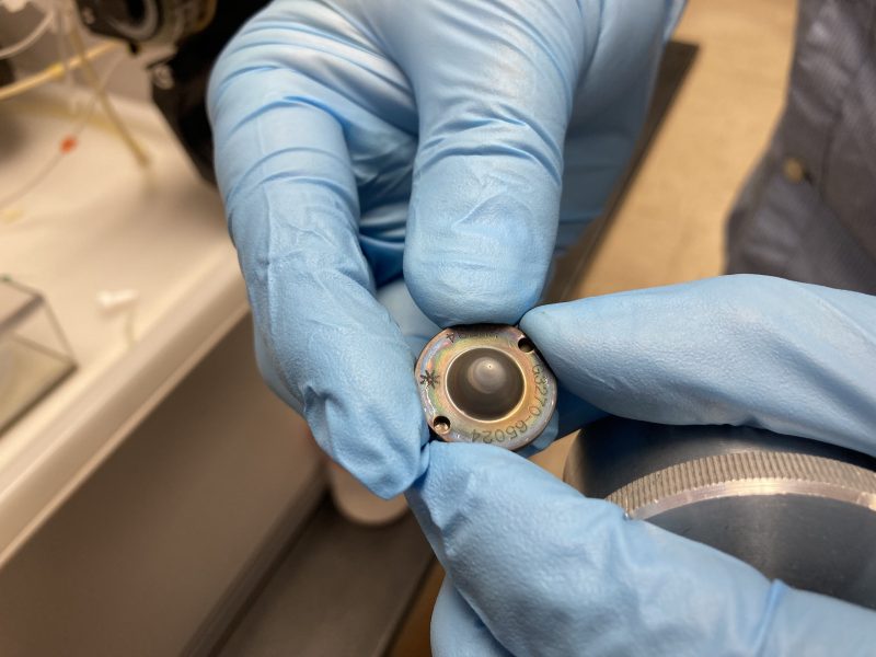
The dirty cone.
Dr. Miller preparing to unbox the new cone.
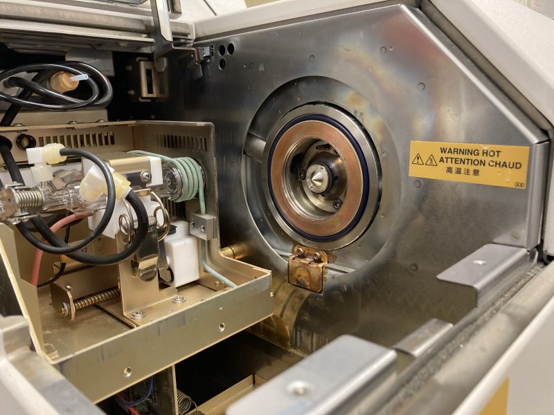
New, clean cone installed in the instrument.
Below are three time lapse videos filmed during data collection. The first two are line scan videos and the third features the creation of one map.
Data Processing: Line scans
I reduced all of the data using the program Iolite. First, the data and scan log .csv files were imported into iolite. I then set up the groups in the timeseries as the baseline, standards, and unknowns from the data, and the best fits were chosen for the baseline and standards. In Data Reduction Schemes, I used NIST610 as the external standard and Si24 as the internal standard. I crunched the data and ran a secondary check in QA/QC using NIST612. All values passed, so I then exported results and statistics as excel files for further processing.
After exporting the excel files, I calculated additional statistics (see Data Quality Information below) from the statistics generated in iolite. To create graphs from the line scans, I calculated the 7 point median and average from the iolite output, and made the final line scan plots using the 7 point average to smooth out to graphs for better readability.
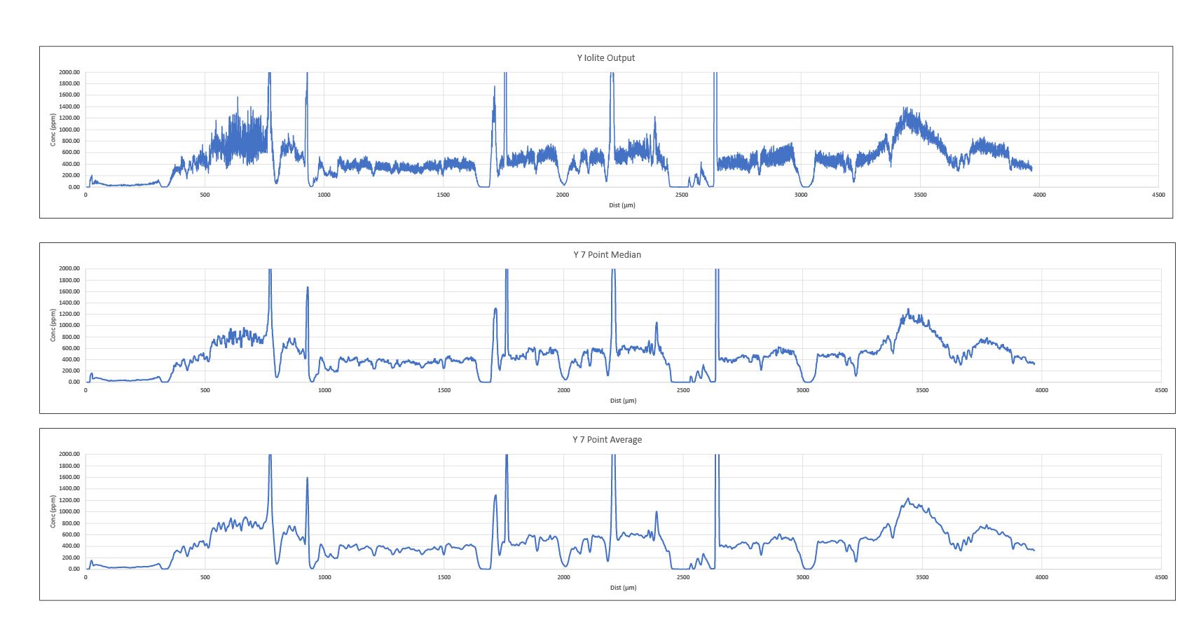
Example of data processing for line scans for Y from R1-R2.
Data Processing: Maps
To reduce the map data, I used the same protocol described above for the line scans with additional steps. After running the secondary check, I generated the maps in Imaging. I selected all unknowns as raster maps and set the width and height to 1000 µm (the size of the maps). I had to rotate the maps to match the orientation of the garnet in my reference photos. Interestingly, both maps were generated in different orientations. I used the spectrum gradient and individually adjusted the upper limits for each map to better reflect the average concentration of each analyte. I tested out different filters but ultimately decided not to apply any of them to my final maps. Finally, I exported the maps as a PDF and created my final figures in Adobe Illustrator.
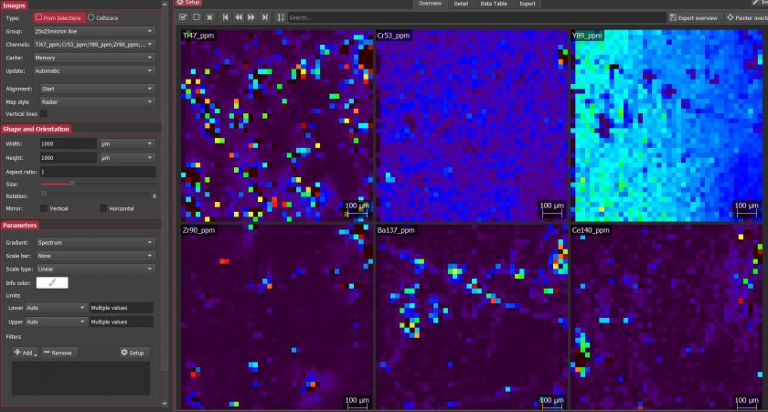
Screenshot of map processing in iolite.
Data Quality Information
Recovery Fractions for Standards run as Unknowns is shown below. The number of analyses for each standard is 6:
|
Analyte |
NIST610 | NIST612 | BHVO | ||||||
| GeoRem Values | Recovery | GeoRem Values | Recovery | GeoRem Values | Recovery | ||||
| ppm | 2SE | ppm | ppm | 2SE | ppm | ppm | 2SE | ppm | |
| Ti | 452 | 10 | 1.0 | 44 | 2.3 | 0.92 | 16300 | 900 | 1.0 |
| Cr | 408 | 10 | 1.0 | 36.4 | 1.5 | 0.99 | 293 | 12 | 1.0 |
| Y | 462 | 11 | 1.0 | 38.3 | 1.4 | 0.99 | 26 | 2 | 1.1 |
| Zr | 448 | 9 | 1.0 | 37.9 | 1.2 | 1.00 | 170 | 7 | 1.2 |
| Ba | 452 | 9 | 1.0 | 39.3 | 0.9 | 1.02 | 131 | 2 | 1.0 |
| Ce | 453 | 8 | 1.0 | 38.4 | 0.7 | 1.01 | 37.6 | 0.2 | 0.9 |
| Eu | 447 | 12 | 1.0 | 35.6 | 0.8 | 1.00 | 2.07 | 0.01 | 1.0 |
| Yb | 450 | 9 | 1.0 | 39.2 | 0.9 | 0.96 | 2.01 | 0.02 | 1.1 |
| Lu | 439 | 8 | 1.0 | 37 | 0.9 | 0.98 | 0.279 | 0.003 | 1.2 |
| Th | 457.2 | 1 | 1.0 | 37.79 | 0.08 | 1.00 | 1.22 | 0.05 | 1.2 |
| U | 461.5 | 1 | 1.0 | 37.38 | 0.08 | 1.02 | 0.403 | 0.003 | 1.0 |
The recoveries for all elements were excellent, either lower than, equal to, or very close to 1.
Typical Elemental Concentrations of Unknowns are shown below and were calculated from the average of each line scan in iolite:
|
Analyte |
Unknowns (n=3) | ||||||
| Average | Max | Min | Median | LOD | Signal-to-Noise | ||
| ppm | 1σ | ppm | ppm | ppm | ppm | ||
| Ti | 2807.4 | 1026.1 | 3837.8 | 1785.7 | 2798.7 | 0.452 | 6211 |
| Cr | 96.8 | 4.2 | 101.3 | 93.2 | 95.8 | 1.313 | 74 |
| Y | 506.4 | 141.3 | 668.3 | 408.0 | 442.9 | 0.012 | 42200 |
| Zr | 110.0 | 93.2 | 211.4 | 28.0 | 90.5 | 0.014 | 7857 |
| Ba | 36.7 | 9.6 | 47.8 | 30.4 | 31.9 | 0.051 | 720 |
| Ce | 130.1 | 180.1 | 335.9 | 1.6 | 52.7 | 0.005 | 26020 |
| Eu | 7.2 | 5.5 | 11.7 | 1.1 | 8.7 | 0.006 | 1200 |
| Yb | 117.4 | 10.3 | 126.9 | 106.5 | 118.8 | 0.017 | 6906 |
| Lu | 25.8 | 3.6 | 29.1 | 22.0 | 26.3 | 0.004 | 6450 |
| Th | 15.0 | 25.8 | 44.8 | 0.0 | 0.2 | 0.005 | 3000 |
| U | 5.0 | 4.1 | 8.9 | 0.7 | 5.4 | 0.003 | 1667 |
Cr had the lowest signal-to-noise value at 74, but all other analytes were either close to or well above 1000x above the detection limit.