Methodology
Pre-analysis
Sample Collection
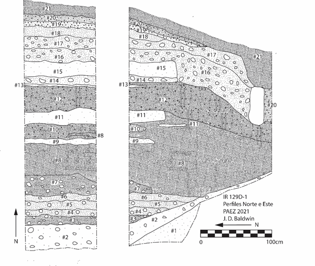
The 21 soil samples were collected in June of 2021 from the excavation unit in the body of the dam. This was done at the conclusion of the season, when the entire stratigraphic sequence could be viewed and assessed. First, we cleaned the profile and sampled each layer using a clean trowel starting from the deepest layer and working our way up to the surface. This was done in order to avoid soil from upper layers contaminating collections made from lower layers. Samples were collected in whirl-pak bags, and subsequently shipped to the Beach Soils and Geoarchaeology Lab at the Department of Geography and the Environment at the University of Texas at Austin.
Sample Preparation
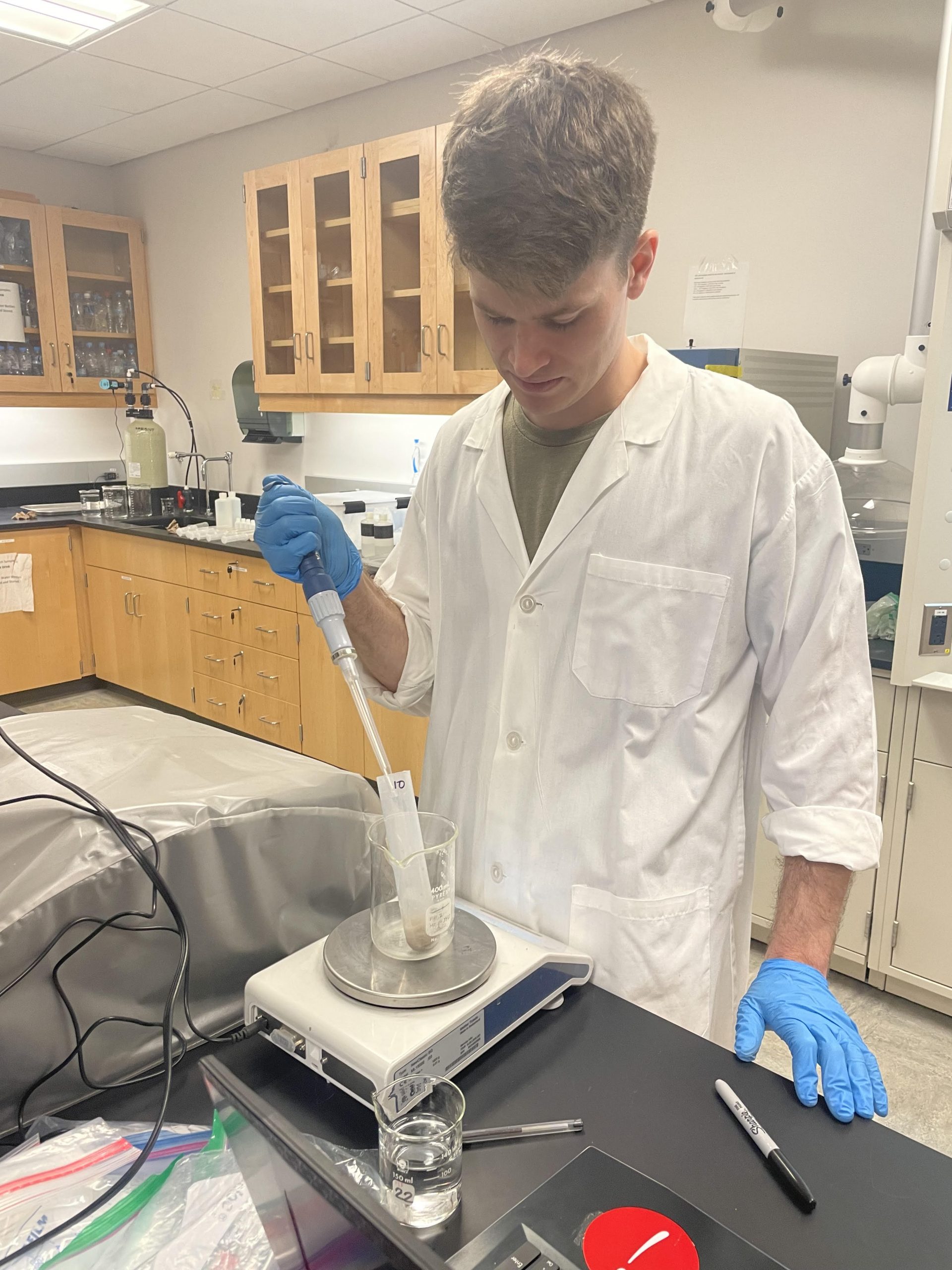
It was first necessary to convert the soils to a form that could be analyzed with the instrument in solution mode. During the sample preparation, I was assisted by my undergraduate research assistant Jamie Rule. We first ground and sifted the 21 samples to 200 microns using a thoroughly cleaned mortar, pestle, and sifter.
Not wanting to totally digest the soil to its most fundamental geological components, I opted for a partial digestion in order to extract the anthropogenic residues within the soil within the leachate. To do this, I adapted a method detailed by Fulton and colleagues (2017, 2019). We combined one gram of each sample with 10 mL of a weak solution made of equal parts HCl (0.6M) and HNO3 (0.16M). Because of the quantity of limestone within the samples, they reacted strongly to the solution, and were left to react under a fume hood for three days.
Once a safe amount of time had passed, the samples were poured into test tubes and run in the centrifuge at 3000 rpms for 20 minutes. The samples were then decanted into a second set of test tubes. At this stage, we judged the samples had too much suspended particulate, so the samples were centrifuged again using a tabletop centrifuge at 3200 rpm for 15 minutes. Subsequently, about 2 mL of each sample was aliquoted into clean vials to be diluted in the ICP-MS lab.
Solution Mode
Semi-quantitative analysis
In order to determine the TDS and approximate concentration of analytes within each sample, I first diluted each to 10x for a semi-quantitative analysis. Consulting with Dr. Miller, we agreed that a 100x dilution would be appropriate (though he felt more comfortable with 1000x, and for good reason!). So these were again diluted 10x. The results indicated that these samples were still too concentrated, and the high concentration of Calcium created significant build-up on the device’s cones (the most concentrated sample was measured to have 330 ppm of Calcium, see below). These findings allowed me to establish appropriate subsequent dilutions to ensure that analyzed samples did not exceed 200ppm going forward. It also allowed me to figure out which analytes I could target in subsequent analyses.
Analytes and Instrument Modes
I selected the following analytes because they are highly attested within the literature as markers of human impacts on the environment (Fulton 2017, 2019). He gas (or collision) mode was selectd for analytes that are prone to interference from large polyatomic ions, while Hydrogen gas (or reaction) mode was selected for analytes sensitive to interfence from more reactive species.
| Isotope | He mode | H2 mode | No gas mode | Int time/mass (s) |
| 23Na | X | 0.3 | ||
| 24Mg | X | X | 0.3 | |
| 27Al | X | 0.3 | ||
| 28Si | X | 0.3 | ||
| 31P | X | 0.3 | ||
| 39K | X | 0.3 | ||
| 40Ca | X | 0.3 | ||
| 43Ca | X | X | 0.3 | |
| 44Ca | X | X | 0.3 | |
| 51V | X | 0.3 | ||
| 52Cr | X | 0.3 | ||
| 53Cr | X | 0.3 | ||
| 55Mn | X | 0.3 | ||
| 56Fe | X | X | 0.3 | |
| 57Fe | X | 0.3 | ||
| 59Co | X | 0.3 | ||
| 60Ni | X | 0.3 | ||
| 63Cu | X | 0.3 | ||
| 66Zn | X | 0.3 | ||
| 88Sr | X | 0.3 | ||
| 107Ag | X | 0.3 | ||
| 137Ba | X | 0.3 | ||
| 206Pb | X | 0.3 | ||
| 207Pb | X | 0.3 | ||
| 208Pb | X | 0.3 | ||
| 238U | X | 0.3 |
Dilutions
Sample Unknowns for the quantitative analysis were diluted in two steps starting with the initial 10x diluted samples created before the semi-quantitative analysis. Based on our results from the semi-quantitative analysis of the 100x samples, I developed new dilution factors to ensure that the TDS levels in the batch were kept at 200ppm to maximize signals of trace elements, while not hurting the machine. Depending on the sample, the refined dilution factors could be as high as 176x or as low as 22x from the original soil leachate.
The second dilution was an arbitrary 20x further dilution of the aforementioned samples, which was done in order to bring Calcium concentrations to within the analytical range of the calibration standards.
Actual dilution factors were key, because they allowed for instrument readings to be converted back to concentrations within the original soil leachate (see results section).
| Sample | Dilution from soil leachate | Dilution to 200ppm | Dilution for major analytes | final dilution from extract |
| 1.2_20x | 9.87 | 17.37 | 19.67 | 3372.77 |
| 2.2_20x | 10.22 | 11.84 | 19.70 | 2383.04 |
| 3.2_20x | 9.58 | 17.57 | 19.66 | 3310.99 |
| 4.2_20x | 9.72 | 18.19 | 19.70 | 3482.71 |
| 5.2_20x | 9.75 | 18.07 | 19.66 | 3465.19 |
| 6.2_20x | 9.84 | 11.61 | 19.70 | 2251.16 |
| 7.2_20x | 9.95 | 9.11 | 19.67 | 1783.70 |
| 8.2_20x | 9.94 | 8.99 | 19.67 | 1757.45 |
| 9.2_20x | 9.81 | 12.48 | 19.59 | 2396.20 |
| 10.2_20x | 9.76 | 7.58 | 19.61 | 1450.50 |
| 11.2_20x | 9.81 | 13.45 | 19.68 | 2597.14 |
| 12.2_20x | 9.85 | 11.39 | 20.25 | 2271.91 |
| 13.2_20x | 9.93 | 9.30 | 19.55 | 1805.77 |
| 14.2_20x | 9.91 | 7.40 | 19.92 | 1461.28 |
| 15.2_20x | 9.94 | 7.82 | 19.49 | 1514.17 |
| 16.2_20x | 10.04 | 5.32 | 19.58 | 1046.15 |
| 17.2_20x | 9.91 | 6.20 | 19.67 | 1208.46 |
| 18.2_20x | 9.98 | 5.71 | 19.58 | 1116.70 |
| 19.2_20x | 10.04 | 3.74 | 19.61 | 736.19 |
| 20.2_20x | 10.10 | 2.52 | 19.70 | 501.76 |
| 21.2_20x | 9.94 | 2.28 | 19.52 | 442.25 |
| 1.1_200ppm | 9.87 | 17.37 | N/A | 171.49 |
| 2.1_200ppm | 10.22 | 11.84 | N/A | 120.99 |
| 3.1_200ppm | 9.58 | 17.57 | N/A | 168.39 |
| 4.1_200ppm | 9.72 | 18.19 | N/A | 176.81 |
| 5.1_200ppm | 9.75 | 18.07 | N/A | 176.22 |
| 6.1_200ppm | 9.84 | 11.61 | N/A | 114.28 |
| 7.1_200ppm | 9.95 | 9.11 | N/A | 90.70 |
| 8.1_200ppm | 9.94 | 8.99 | N/A | 89.33 |
| 9.1_200ppm | 9.81 | 12.48 | N/A | 122.34 |
| 10.1_200ppm | 9.76 | 7.58 | N/A | 73.98 |
| 11.1_200ppm | 9.81 | 13.45 | N/A | 131.98 |
| 12.1_200ppm | 9.85 | 11.39 | N/A | 112.17 |
| 13.1_200ppm | 9.93 | 9.30 | N/A | 92.36 |
| 14.1_200ppm | 9.91 | 7.40 | N/A | 73.35 |
| 15.1_200ppm | 9.94 | 7.82 | N/A | 77.69 |
| 16.1_200ppm | 10.04 | 5.32 | N/A | 53.44 |
| 17.1_200ppm | 9.91 | 6.20 | N/A | 61.44 |
| 18.1_200ppm | 9.98 | 5.71 | N/A | 57.02 |
| 19.1_200ppm | 10.04 | 3.74 | N/A | 37.54 |
| 20.1_200ppm | 10.10 | 2.52 | N/A | 25.47 |
| 21.1_200ppm | 9.94 | 2.28 | N/A | 22.66 |
Instrument Parameters:
The instrument was operated using the following parameters:
| Plasma Parameter | |
| RF Power | 1600 V |
| RF Matching | 1.7 V |
| Sample Depth | 8.5 mm |
| Torch-H | 0.4 mm |
| Torch-V | -0.4 mm |
| Carrier Gas | 0.88 L/min |
| Makeup Gas | 0.33 L/min |
| Nebulizer pump | 0.10 rps |
| S/C temp | 2 C |
| Ion Lenses | |
| Extract 1 | 3.0 V |
| Extract 2 | -155.0 V |
| Omega Bias-ce | -22 [-22] V |
| Omega Bias-ce | 2.8 [2.8] V |
| Cell Entrance | -40 [-30] V |
| QP Focus | 2 V |
| Cell Exit | -60 [-50] V |
| Quadrupole Parameters | |
| AMU Gain | 126 |
| AMU Offset | 128 |
| Axis Gain | 0.9999 |
| Axis Offset | 0 |
| QP Bias | -13.0 [-3.0] V |
| Octopole Parameters | |
| Octopole RF | 190 V |
| Octopole Bias | -16.0 [-6.0] V |
| Reaction Cell | |
| H2 gas | 4.5 mL/min |
| He gas | 5.0 mL/min |
| Detector Parameters | |
| Discriminator | 8 mV |
| Analog HV | 1750 V |
| Pulse HV | 1360 V |
Analytical Order
First, an initial washout of the machine was performed before the L1 through L6 calibration standards to ensure that background contamination was minimized. After the L6 standard, five blanks were run before replicates of the quality control (QC) standards. Thereafter, a quick washout with two blanks minimized contamination of the unknowns. After careful consideration, it was decided to run the more dilute (20x) samples first in order to maximize the instrument’s sensitivity and prevent the more concentrated samples from clogging the instrument’s interface. After every 10 samples, two blanks bracketed a QC, which were alternated between the NIST 1643f and the L4 B standard.
| Run # | Sample |
| 1 | fake blank |
| 2 | fake blank |
| 3 | fake blank |
| 4 | HNO3 blank (L1) |
| 5 | Cal Std A L2 |
| 6 | Cal Std A L3 |
| 7 | Cal Std A L4 |
| 8 | Cal Std A L5 |
| 9 | Cal Std A L6 |
| 10 | HNO3 blank |
| 11 | HNO3 blank |
| 12 | HNO3 blank |
| 13 | HNO3 blank |
| 14 | HNO3 blank |
| 15 | QC1 (NIST 1643f) |
| 16 | QC1 (NIST 1643f) |
| 17 | QC2 (Cal Std B L4) |
| 18 | QC2 (Cal Std B L4) |
| 19 | HNO3 blank |
| 20 | HNO3 blank |
| 21 | 1.2_20x |
| 22 | 2.2_20x |
| 23 | 3.2_20x |
| 24 | 4.2_20x |
| 25 | 5.2_20x |
| 26 | 6.2_20x |
| 27 | 7.2_20x |
| 28 | 8.2_20x |
| 29 | 9.2_20x |
| 30 | 10.2_20x |
| 31 | HNO3 blank |
| 32 | QC1 (NIST 1643f) |
| 33 | HNO3 blank |
| 34 | 11.2_20x |
| 35 | 12.2_20x |
| 36 | 13.2_20x |
| 37 | 14.2_20x |
| 38 | 15.2_20x |
| 39 | 16.2_20x |
| 40 | 17.2_20x |
| 41 | 18.2_20x |
| 42 | 19.2_20x |
| 43 | 20.2_20x |
| 44 | HNO3 blank |
| 45 | QC2 (Cal Std B L4) |
| 46 | HNO3 blank |
| 47 | 21.2_20x |
| 48 | 1.1_200ppm |
| 49 | 2.1_200ppm |
| 50 | 3.1_200ppm |
| 51 | 4.1_200ppm |
| 52 | 5.1_200ppm |
| 53 | 6.1_200ppm |
| 54 | 7.1_200ppm |
| 55 | 8.1_200ppm |
| 56 | 9.1_200ppm |
| 57 | HNO3 blank |
| 58 | QC1 (NIST 1643f) |
| 59 | HNO3 blank |
| 60 | 10.1_200ppm |
| 61 | 11.1_200ppm |
| 62 | 12.1_200ppm |
| 63 | 13.1_200ppm |
| 64 | 14.1_200ppm |
| 65 | 15.1_200ppm |
| 66 | 16.1_200ppm |
| 67 | 17.1_200ppm |
| 68 | 18.1_200ppm |
| 69 | 19.1_200ppm |
| 70 | 20.1_200ppm |
| 71 | 21.1_200ppm |
| 72 | HNO3 blank |
| 73 | QC2 (Cal Std B L4) |
| 74 | HNO3 blank |
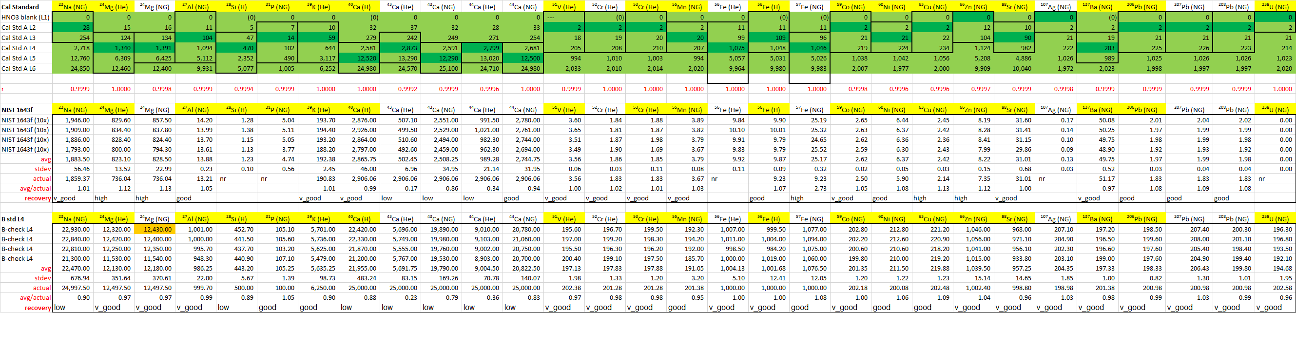
Data Quality
Calibration standards bracket the measured unknowns very well, and r-scores are all very close to 1. The NIST 1643f (10x) standard does not serve as a quality control for all of the target analytes, but luckily the B L4 calibration standard provides validation for 28Si, 31P, and 238U. Analytes that were chosen for analysis are highlighted in yellow. These are: 23Na, 24Mg, 27Al, 28 Si, 31P, 39K, 40Ca, 51V, 53Cr, 55Mn, 56Fe, 59Co, 60Ni, 63Cu, 66Zn, 88Sr, 137Ba, 206Pb, and 238U. Despite fine calibration values for 107Ag, measured values in both of the dilutions were below the LOD calculated for that analyte so 107Ag was excluded from the final analysis.