Methodology
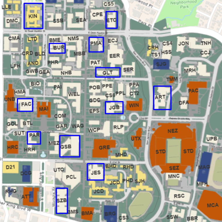
As previously mentioned, we collected two samples each from twelve different buildings (at different floor levels) to account for variation across campus and variation from floor to floor. We tested the following buildings: ETC, PMA, GLT, JGB, GSB, KIN, FAC, PAR, BUR, ART, SZB, and JES. We utilized inductively coupled plasma mass spectrometry, also known as ICP-MS, to test for contaminants in the water. We mixed the water samples with stability solutions to create liquid solutions, which we then tested using ICP-MS technology.
We analyzed the data according to two standards. The first is the EPA standards for each respective element, using Method 200.8 from the EPA for ICP-MS. The second method is the ISO 17294-2 method using collision reaction cells (CRC), a technique in which kinetic energy discrimination is used to reduce interferences, allowing for precise testing of trace elements. While many drinking water analyses use Method 200.8, collision reaction cells efficiently reduce interferences without the use of interference equations. We looked into whether or not the two methods for each metal are significantly different.
Using an Agilent 7500ce ICP-Q-MS at the University of Texas at Austin (Department of Geological Sciences), we determined (11/30/23) cation concentrations (Sc, V, Ni, Cu, Zn, As, Se, Y, Cd, In, Te, Pb, Bi). We optimized the instrument for sensitivity across the AMU range while minimizing oxide production (CeO/Ce < 1.05%). The quantitative-analytical method employed an octopole reaction system (ORS), operated in both helium (collision mode) and hydrogen (reaction mode) for the removal of polyatomic interferences. We used internal standards, mixed into unknowns via in-run pumping, to compensate for instrumental drift. Internal standard sensitivity variations fell well within QA tolerances (60% to 160%). Limits of detection, based upon the population of blank (2% HNO₃) analyses interspersed throughout the analytical sequence were typically better than 0.01162 ppb (median = 0.08647 ppb) for analytes measured in optimal modes (with or without the ORS). Analyte recoveries obtained for replicates of two independent quality control standards were typically within 4% of certified values. Relative precisions (n = 24) obtained for these quality control standards were typically within 1 to 3% of replicate averages. ICP-MS analytical parameters are shown in the following tables.
| ICP-MS Instrument | Agilent 7500ce ICP-Q-MS |
| Plasma Conditions | |
| Nebulizer | PFE microflow with 90 µL/min uptake rate |
| Nebulizer pumps (rps) | 0.2 |
| Spray Chamber | Scott-type (quartz) with Peltier cooling (2°C) |
| Sampling Depth (mm) | 8 |
| RF Power (W) | 1600 |
| RF Matching (V) | 1.7 |
| Carrier gas flow (L/min) | 0.85 |
| Make-up gas flow (L/min) | 0.35 |
| Cones | Ni |
| Reaction cell (ORS) modes and masses measured | |
| He mode (5.3 mL/min) | 51, 52, 53, 63, 65, 75, 78, 89 |
| H₂ mode (3.3 mL/min) | 45, 78, 89 |
| No gas mode | 45, 51, 52, 53, 60, 62, 63, 65, 66, 68, 75, 77, 82, 83, 89, 106, 108, 111, 114, 115, 118, 125, 206, 207, 208, 209 |
| Internal stds | 45, 89, 115, 125, 209 |
| Detection system | Dual stage (pulse & analog) discrete dynode electron multiplier |
| Data Acquisition | |
| Scan mode | Peak hopping |
| Points across peak | 3 |
| Integration per mass (sec) | 0.100 |
| Replicates | 3 |
Table 1: Operating Conditions and Instrument Parameters
| Step | Mode | Flow | Cell Entrance | Cell Exit | OctP Bias | QP Bias |
| 1 | Helium | 5.3 mL/min | – 40 V | – 60 V | – 16 V | – 13 V |
| 2 | Hydrogen | 3.3 mL/min | – 40 V | – 60 V | – 16 V | – 13 V |
| 3 | No Gas | N/A | – 30 V | – 50 V | – 6 V | – 3 V |
Table 2: Summary of Methods
We then analyzed the elements using the methods mentioned above. The acquisition mode is Spectrum Analysis (Multi-Tune) and the number of masses is twenty-seven. Here is an alternate view of the elements measured; each column contains an “x” mark for which method we used to record that element using ICP-MS technology:
| Mass | Element | Integration Time (s) | Helium [#1] | Hydrogen [#2] | No Gas [#3] |
| 45 | Sc | 0.30000 | x | x | x |
| 51 | V | 0.10000 | x | x | |
| 52-53 | (V) | 0.10000 | x | x | |
| 60 | Ni | 0.10000 | x | ||
| 62 | Ni | 0.10000 | x | ||
| 63 | Cu | 0.10000 | x | x | |
| 65 | Cu | 0.10000 | x | x | |
| 66 | Zn | 0.10000 | x | ||
| 68 | Zn | 0.10000 | x | ||
| 75 | As | 0.10000 | x | x | |
| 77 | (As) | 0.10000 | x | ||
| 78 | Se | 0.10000 | x | ||
| 82-83 | (As) | 0.10000 | x | ||
| 89 | Y | 0.30000 | x | x | x |
| 106 | Cd | 0.10000 | x | ||
| 108 | Cd | 0.10000 | x | ||
| 111 | Cd | 0.10000 | x | ||
| 114 | Cd | 0.10000 | x | ||
| 115 | In | 0.30000 | x | ||
| 118 | (In) | 0.10000 | x | ||
| 125 | Te | 0.30000 | x | ||
| 206-208 | Pb | 0.10000 | x | ||
| 209 | Bi | 0.30000 | x |
Table 3: Elements Measured in Different Analysis Modes
Internal standards have an integration time of 0.30000 seconds, while analytes have an integration time of 0.10000 seconds.
| m/z | Element | Range | Count | Mean | RSD% |
| 45 | Scandium | 5,000,000 | 578400.0 | 597169.5 | 2.64 |
| 89 | Yttrium | 2,000,000 | 202416.0 | 203398.9 | 1.95 |
| 115 | Indium | 1,000,000 | 141103.0 | 139171.0 | 1.73 |
| 125 | Tellurium | 100,000 | 9680.0 | 9707.5 | 2.05 |
| 209 | Bismuth | 1,000,000 | 109017.0 | 109611.2 | 1.61 |
Table 4: Final Tune Results
The relative standard deviations (RSD%) for the internal standards are within reasonable ranges.
| Step | Mass | Element | r | a | b(blank) | c | DL | BEC | Unit |
| 1 | 51 | V | 1.0000 | 2.98E-02 | 6.77E-05 | 0 | 1.18E-02 | 2.28E-03 | ppb |
| 3 | 51 | V | 1.0000 | 7.32E-03 | 3.44E-04 | 0 | 4.95E-03 | 4.70E-02 | ppb |
| 1 | 52 | V | 1.0000 | 4.17E-02 | 1.36E-03 | 0 | 1.68E-02 | 3.25E-02 | ppb |
| 3 | 52 | V | 1.0000 | 6.24E-03 | 1.94E-03 | 0 | 3.23E-02 | 3.11E-01 | ppb |
| 1 | 53 | V | 1.0000 | 5.01E-03 | 3.40E-04 | 0 | 1.86E-01 | 6.77E-02 | ppb |
| 3 | 53 | V | 1.0000 | 7.32E-04 | 1.39E-04 | 0 | 3.34E-02 | 1.90E-01 | ppb |
| 3 | 60 | Ni | 1.0000 | 1.47E-03 | 2.96E-04 | 0 | 3.86E-02 | 2.02E-01 | ppb |
| 3 | 62 | Ni | 1.0000 | 2.14E-04 | 5.92E-04 | 0 | 3.43E-01 | 2.77E+00 | ppb |
| 1 | 63 | Cu | 1.0000 | 5.91E-02 | 9.49E-04 | 0 | 4.30E-02 | 1.61E-02 | ppb |
| 3 | 63 | Cu | 1.0000 | 3.21E-03 | 5.53E-05 | 0 | 6.99E-03 | 1.72E-02 | ppb |
| 1 | 65 | Cu | 1.0000 | 2.89E-02 | 2.71E-04 | 0 | 3.23E-02 | 9.38E-03 | ppb |
| 3 | 65 | Cu | 1.0000 | 1.49E-03 | 2.13E-05 | 0 | 3.24E-03 | 1.43E-02 | ppb |
| 3 | 66 | Zn | 1.0000 | 4.82E-04 | 7.41E-05 | 0 | 2.53E-02 | 1.54E-01 | ppb |
| 3 | 68 | Zn | 1.0000 | 3.36E-04 | 1.06E-04 | 0 | 7.75E-02 | 3.15E-01 | ppb |
| 1 | 75 | As | 1.0000 | 6.77E-03 | 0 | 0 | — | 0 | ppb |
| 3 | 75 | As | 1.0000 | 4.16E-03 | 2.18E-05 | 0 | 1.48E-03 | 5.23E-03 | ppb |
| 3 | 77 | Se | 1.0000 | 3.33E-05 | 1.13E-05 | 0 | 1.37E-01 | 3.39E-01 | ppb |
| 1 | 78 | Se | 0.0000 | — | — | — | — | — | ppb |
| 2 | 78 | Se | 1.0000 | 9.89E-05 | 0 | 0 | — | 0 | ppb |
| 3 | 78 | Se | 1.0000 | 1.07E-04 | 9.15E-04 | 0 | 9.16e-1 | 8.57 | ppb |
| 3 | 82 | Se | 1.0000 | 4.32E-05 | 8.98E-06 | 0 | 3.69E-01 | 2.08E-01 | ppb |
| 3 | 106 | Cd | 1.0000 | 4.62E-03 | 3.40E-02 | 0 | 1.247 | 7.364 | ppb |
| 3 | 108 | Cd | 1.0000 | 3.34E-03 | 2.53E-03 | 0 | 1.69E-01 | 7.57E-01 | ppb |
| 3 | 111 | Cd | 1.0000 | 5.03E-02 | 2.78E-04 | 0 | 1.71E-02 | 5.53E-03 | ppb |
| 3 | 114 | Cd | 1.0000 | 1.18E-01 | 6.58E-04 | 0 | 4.48E-03 | 5.57E-03 | ppb |
| 3 | 206 | Pb | 0.9999 | 2.12E-03 | 1.41E-05 | 0 | 3.00E-03 | 6.66E-03 | ppb |
| 3 | 207 | Pb | 1.0000 | 1.71E-03 | 1.23E-05 | 0 | 4.88E-03 | 7.22E-03 | ppb |
| 3 | 208 | Pb | 1.0000 | 8.18E-03 | 5.32E-05 | 0 | 1.53E-03 | 6.52E-03 | ppb |
Table 5: Calibration Results
The calibration results rho (r) fall within 0.9999 to 1.0000, showing high recovery fractions.