Methodology

Sample Collection and Preparation

Rock fragments were sampled from the UT BEG repository of cores collected during well drilling at Mirasol Springs and Reimer’s Ranch. Five samples were selected for analysis; one from each geologic unit of interest: the Lower Glen Rose Limestone, Hensel Sand, Cow Creek Limestone, Hammett’s Shale, and Sycamore Sand (a strat column, study area map and images of the rock samples can be found on the proposal page).

Samples were powdered using an agate mortar and pestle, then digested using two separate methods: one to isolate just the carbonate fraction of each rock, and the other to dissolve the whole rock.

• Carbonate fraction: About 100mg of sample was added to a 2mL microcentrifuge tube. A 1.5mL solution of 0.2M ammonium acetate (pH 8) was added to the tube, which is used to dissolve only the CaCO3 fraction of the rock. The mixture was shaken and left to react for 5 minutes. It was then centrifuged for a minute, after which the liquid was decanted from the solid. This process was repeated twice with the 0.2M ammonium acetate solution, after which it was repeated three times with twice-distilled water. To isolate the carbonate fraction, 1.5mL of 4% acetic acid was added to the remaining solid and shaken, then left to react for 10 minutes. The mixture was centrifuged, and the decanted liquid was added to a beaker along with 1mL of 6N nitric acid. The samples were left to dry on a hot plate over night. The next day, 0.2-0.3 mL of 6N nitric acid was added to the samples and they were again left to dry. The remaining residue was rinsed with twice-distilled water, centrifuged, and the remaining liquid was decanted. The samples were rinsed in this manner twice. The solution was left to dry, and was then brought up in (vol?) 3M nitric acid.
• Whole rock: HF and HNO3 were added to the samples and digested in a microwave digestor. The samples were then dried and brought up in acid then dried again. The samples were dissolved and dried until the entirety of the sample could dissolve, at which point they were dried again and finally dissolved in 3M HNO3 to be further diluted and analyzed via solution mode ICP-MS.

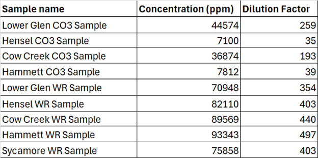
After each sample was dissolved, they were diluted to about 200ppm total dissolved solids. To do so, the approximate TDS was calculated for each sample by dividing the mass of sample (for WR) or mass of CO3 residue (for CO3) by the mass of final solution. The samples were then gravimetrically diluted using 2% nitric acid to about 200ppm TDS. The required volumes of sample and acid were pipetted and weighed, and the actual dilution factor was calculated by dividing the calculated volume (mass/density) of added sample by the total volume of the sample and acid (Table 1). The samples were then ready for analysis.

Blanks

Method Blanks

Method blanks are used to measure contamination during sample collection and/or preparation. A method blank was created for each of the two rock digestion methods (one for the carbonate digestion and the other for the whole rock digestion). These blanks ran through all of the same digestion steps as the rock samples, except they contained no rock material. At the end of the rock digestion process, each sample was diluted with nitric acid, meaning the blank should theoretically only contain nitric acid, and should show 0 REE concentration (should all be below detection).

Instrument Blanks

Instrument blanks were also used to ensure that any contaminants introduced during the running of the ICPMS can be accounted for. Instrument blanks were run between each group of standards and unknowns. These blanks are used to determine the limit of detection of the instrument, which can be calculated for each element by multiplying it’s average concentration by the TINV (using a probability of .05). Any concentration measurements falling below the limit of detection cannot be reported as accurate.

Standard Preparation

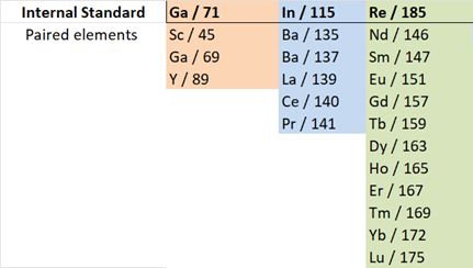
Internal Standards: An internal standard solution of Ga, In and Re was added (in-run) to diluted samples. Internal standards are important because they allow us to account for instrument drift. The signal of each internal standard should remain the same throughout the run, however natural instrument drift causes the signals to fluctuate slightly. Calculating the drift factors and multiplying all signals by their respective drift factors helps to remove error/deviations in signal measurements due to drift. Re, In and Ga were selected as standards based on how close their masses are to the REE masses whose drift is being corrected. Table 2 shows which internal standards were paired to which elements of interest.

Calibration Standards: Two multi-element stock solutions were diluted with 2% nitric acid to create calibration standards: one containing just Ba and another containing all REEs. The solutions were diluted at 6 different dilution factors to ideally bracket the REE and Ba concentrations in the diluted unknown samples. Calibration standards are used to calculate the concentrations of each element from their signal. If we know the actual concentration of the standard and can compare it to its measured signal, we can relate signals to concentrations (with calibration curves). It is important that these calibration curves have a high linearity and high r value to ensure that the calibration curves are accurate enough to be useful.

Quality Control Standards: A separate REE stock (different from calibration stock) was diluted to create a 10ppb quality control standard. The Ba single element standard was used as the Ba quality control standard. These standards were used to assess accuracy and precision of the final results.

Single Element Standards: Following Negrel et al. (2000), single element solutions of ~100 ppb Nd, Pr, Sm, Ce, Gd, Eu, Tb, and Ba were made from custom standards acquired for the project. Single element standards are very important for REE analysis using Q-ICP-MS because they allow us to remove oxide and hydroxide interferences via interference equations. The elements used for single element standards are selected based on the elements that create interferences on REE’s.

Instrument Optimization and Analysis

Instrument conditions were tuned to be suitable for REE analysis. The following isotopes were selected for analysis: 45Sc, 89Y, 135Ba, 137Ba, 139La, 140Ce, 141Pr, 146Nd, 147Sm, 151Eu, 157Gd, 159Tb, 163Dy, 165Ho, 167Er, 169Tm, 172Yb, and 175Lu. Internal standard elements were delineated as 71Ga, 115In and 185Re in the program. Instrumental parameters were all kept the same between the runs, except for the carrier gas flow rate (Figure 1). For each run, no gas mode was used on the CRC because neither He nor H gasses are effective in removing REE interferences due to their high masses. During tuning, the omega lens bias was adjusted to increase sensitivity over the AMU mass range of the REEs.

For the low oxide production tune, the carrier gas rate was set to 0.82 L/min, which decreased the ratio of CeO/Ce (m/z 156/140) to about 1%. For the high oxide production tune, the carrier gas rate was set to 0.90 L/min, which raised the CeO/Ce ratio to 3.8%. After all parameters had been set, the samples and standards were analyzed, first with the oxide tune and then with the low oxide tune; completely through twice (once for each tune).

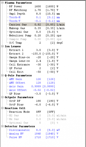
Figure 1: List of the parameters set for the low oxide tune run. All of the parameters were the same for the high oxide tune except the carrier gas (highlighted in grey) was set to 0.90 L/min.

Data Reduction

After analysis, REE signal intensities from both tune runs were corrected for drift, blanks, and MO⁺/MOH⁺ interferences before converting to concentrations and assessing quality. The data reduction steps are detailed below and in the downloadable spreadsheet:

1. Drift correction
2. Blank subtraction
3. Calculation of MO+/M+ and/or MOH+/M+ production ratios, adjusted for isotopic abundance
4. Interference summation & subtraction
5. Converting corrected intensities to concentrations
6. Determination of data quality metrics (LODs, regression r-values, quality control standard recoveries)
7. Adjusting sample concentrations for dilution factors

In the spreadsheet, Steps 1 and 2 are performed on the tab labeled “Correct for Drift”. Steps 3-8 are completed separately on corresponding tabs for the high and low oxide production tunes.

Step 1: Drift Correction

Analyte intensities were corrected for instrumental drift using specific internal standard elements (bolded below):

• 71Ga: 45Sc, Y89
• 115In: 135Ba, 137Ba, 139La, 140Ce, 141Pr
• 185Re: 146Nd, 147Sm, 151Eu, 157Gd, 159Tb, 163Dy, 165Ho, 167Er, 169Tm, 172Yb, 175Lu

Baseline intensities were established from the internal standards measured in the initial calibration blank. For subsequent runs, deviations in internal standard intensities were used to adjust the linked analyte signals. For example, if 71Ga increased by 5% in a later run, intensities for 45Sc and Y89 were corrected by multiplying by 0.95.

Step 2: Blank Subtraction

Analyte intensities were adjusted by subtracting the amount necessary to bring the calibration blank value to zero.

Step 3: Calculate Oxide Production Factors, Weighted for Isotopic Abundances

Interference from MO⁺ and MOH⁺ species (from Ba and certain REEs) was only considered for analyte masses ≥146 (see Table 4).

Isotopes of Ba, Ce, Pr, Nd, Sm, Eu, Gd, and Tb were analyzed for their contributions to oxide/hydroxide interferences, occurring at +16 or +17 m/z, respectively. Production ratios (MO⁺/M⁺ and MOH⁺/M⁺) were calculated from single-element standards and adjusted for isotopic abundance differences between the interfering and measured isotopes.

Example: To correct for 130BaOH⁺ interference on m/z 147 (targeting 147Sm), the 147/137Ba signal ratio is adjusted using isotopic abundances:
Production ratio = (147cps / 137cps) × (0.106 / 11.23)
This ratio is then multiplied by 137Ba intensity in the sample to estimate interference. Where multiple interferences affect the same analyte mass, each contribution is calculated separately and summed.

Step 4: Interference Summation & Subtraction

Interference values from Step 3 were summed for each analyte m/z. These totals were compared with measured intensities to assess the size of the interference correction. The summed interference intensity was subtracted from the Step 2 values to yield corrected analyte intensities.

Step 5: Calculate calibration curves and convert signals to a concentration

Calibration curves were generated using standard concentrations and interference-free signals to determine slope, intercept, and correlation (r). Final concentrations (ppb) were calculated using the equation y = mx + b, where x is the corrected signal.

Step 6: Calculate limits of detection

LOD values were determined from replicate blanks (n=12, 2% HNO₃). The LOD was calculated as:
LOD = standard deviation × t-value (95% confidence), using Excel’s T.INV function.
Replicate QC standards (n=3) were used to assess analytical precision and accuracy.

Step 7: Adjust sample concentrations

Final concentrations were scaled using dilution factors from sample prep (e.g., digestion and dilution for ICP-MS). Results were reported in ppm to enable normalization against NASC (North American Shale Composite) and visualization in REE spider diagrams.