Discussion
Discussion of Results
2D Maps and Zoning
Prior to running any LA-ICP-MS scans, one hypothesized theory about the spherules is that they would exhibit zoning. This is because some of them had an almost ooid like appearance, with concentric rings visible within reflected light (RL). However, this could not be confirmed as compositional zoning based on RL alone due to lack of trace element data, alongside there being a wide array of spherules with different growth patterns and appearances. While some appeared zoned, others countered this through a more radial appearance, supporting the idea of transport being responsible for the zoned appearance rather than growth.
Figure 6.1: Molybdenite spherule with zoned appearance.
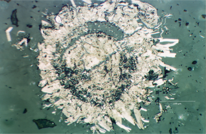
Figure 6.2: Molybdenite spherule with radial appearance.
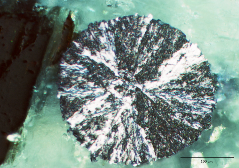
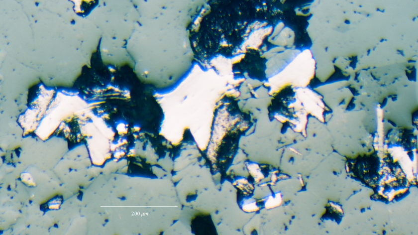
Figure 6.3: Typical bladed Cave Peak molybdenite.
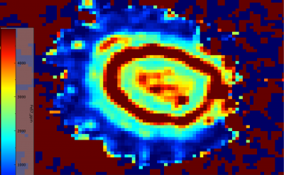
The 2D maps demonstrate notable zoning amongst some elements within the molybdenite spherules. Not all elements exhibited zoning, with some staying relatively consistent throughout the spherule such as 65Cu which is absent throughout. However, most elements scanned within the raster map did show some degree of zoning. The strongest zoning was present in 57Fe and 77Se. 57Fe showed several concentric rings with significant concentration variation between them. The most exterior portions of the spherule are low in 57Fe, these areas appeared more bladed in texture, and this may support the idea of this exterior bladed-like surface being a later growth of molybdenite on an already existing molybdenite core. 77Se does not show such concentric zoning, but rather a strong difference in concentration between the spherule center and the exterior portions, with the center being very low in 77Se while the exterior portions are very high in 77Se. This further supports the idea that in the exterior, bladed-like areas of the spherule are later growths of molybdenite that seeded off of an already existing spherule, therefore, growing in a different environment with different melt compositions and trace element compatibilities. The remainder of the elements somewhat show a lesser degree of zoning. Most of them show weak concentric rings of zoning stretching outward from the spherule center, with more notable concentration differences in the exterior portions of the molybdenite grain. 60Ni, 93Nb, 182W, 204Pb, and 57Fe all have lower concentrations in the exterior portions of the grain than spherule core, with only 77Se being more enriched in the exterior zone.
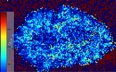
While not as strong of zoning as the spherule, the bladed/typical molybdenite grain also exhibits some weak zoning amongst some elements. Fewer elements exhibit zoning in this grain than within the spherule, with 182W, 204Pb, and 65Cu either not exhibiting any zoning or it being so weak that it cannot be differentiated. However, 77Se still exhibits very strong zoning, inverse of the pattern seen within the spherule. Within the typical molybdenite grain, 77Se shows an odd, double core structure. This comprises of two separate spherical concentrations which are enriched in 77Se relative to the rest of the grain which progressively drops in 77Se concentration outward. The remaining elements, those being 57Fe, 93Nb, and 60Ni all show some degree of zoning around this double core too, though it is much weaker. 57Fe and 93Nb show the opposite of 77Se, with low concentrations within each of the double cores and marginally higher values outlining them. 60Ni has the weakest zoning, with rings of marginally higher concentration outlining the double core feature before dropping back down in concentration toward the grain rims.
It should be noted that many of the elements high in concentration within the spherule core and low in its rims show inverse relationships within the typical molybdenite, being low in the core and higher in concentration closer to the rims (57Fe, 93Nb, and 60Ni). At the same time, 77Se shows an opposite correlation to this, with low concentration within the spherule’s core but high in the rims, while having high concentrations within the double core of the typical molybdenite and lower concentrations in the rims.
Below are side by side images of 57Fe and 77Se within each map.
Figure 6.4: Zoning of 77Se in spherule (top). Zoning of 77Se in typical molybdenite grain (bottom).
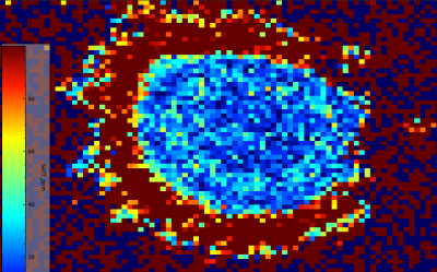
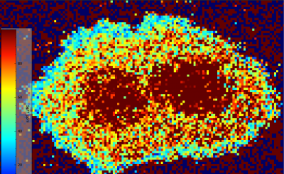
Figure 6.5: Zoning of 57Fe within spherule (top). Weak but still present zoning of 57Fe within typical molybdenite grain (bottom).
Line Scans
The line scans were broken down into four separate aforementioned categories. The primary focus of this discussion will be between ‘Typical Molybdenite’ and ‘Spherule Molybdenite’ as the two other categories are smaller in data pool and are of more questionable value and/or representation.
Line Scan Result Overview
The trace element composition between spherules and typical molybdenite varied significantly, with some variance being greater than others. The only element that is roughly the same in average concentration between spherules and typical molybdenite is 107Ag (51.3 vs. 55.5 ppm). However, all other elements favored, often strongly, either one habit or the other. Elements that were preferentially taken in by typical/bladed molybdenite is 65Cu, 77Se, 182W, 187Re, 238U and total Pb. Spherical molybdenite preferentially took in 57Fe, 59Co, 60Ni, 75As, 118Sn, 121Sb, and 209Bi. Elements that showed the strongest degrees of preferential enrichment (>2.5x concentration enrichment) were 59Co, 60Ni, 75As, and 209Bi which strongly favor spherical molybdenite while 238U and Total Pb were strongly favored in typical molybdenite at Cave Peak.
It should be noted that 209Bi was strongly enriched within both types of molybdenite at Cave Peak compared to previous molybdenite LA-ICP-MS studies. Concentrations at Cave Peak averaged 2382ppm for typical molybdenite and 9536ppm in spherical molybdenite with peaks as high as 41632ppm for lines. This is a significant bismuth enrichment. Previous studies that used LA-ICP-MS to analyze bismuth in molybdenite found values akin to 530ppm 209Bi for the highest average across samples (Ciobanu et al. 2013).
Relative Enrichment and Geochemical Import
Molybdenite found within porphyry deposits, such as Cave Peak (Porphyry-Mo) tends to be most enriched in Re, Cu, Ag, Se, Pb, Bi, and Te while all other common Mo deposit types are generally relatively more enriched in Ni, Co, Sn, and W (Tan et al. 2023). Cave Peak is a porphyry-Mo deposit, and should expect to see enrichment patterns similar to other porphyry deposits. However, this relationship between trace elements in molybdenite and deposit type can speak to the conditions within a deposit during mineralization required to enrich in each respective element. If one type were to be more enriched in one of these elemental groups over another, it may mean that its mineralizing conditions are more or less like those expected during typical porphyry molybdenite mineralization.
Relative relationships between elements can reveal enrichment trends during mineralization shedding new light beyond what a spreadsheet alone can demonstrate. To better understand the relationships between elements, it is vital to be able to plot multiple elements against each other relative to concentration simultaneously as is done in the following triangular plots.
Cobalt is generally more relatively enriched with molybdenite found in non porphyry type deposits. In the first set of 3 triangular plots, 59Cu was kept static as a point of reference for changing relative concentrations within the molybdenite.
Figure 6.6: Co-Re-Sb Triangle Plot
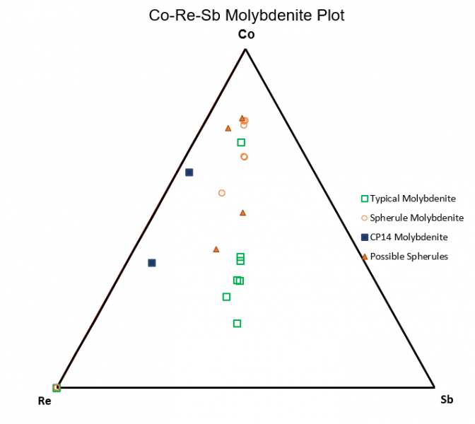
Figure 6.7: Co-W-Sb Triangle Plot
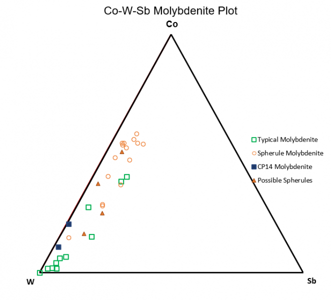
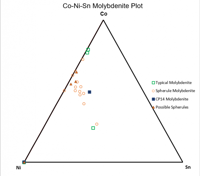
Figure 6.8: : Co-Ni-Sn Triangle Plot
Of note, figure 6.6 shows cobalt being more compatible within spherule molybdenite while rhenium and antimony are relatively more compatible within typical molybdenite. Figure 6.7 continues to show this same trend of cobalt being more compatible within spherule Mo while tungsten strongly favors typical molybdenite. Antimony has similar relatively compatibilities in each habit when compared to against Co and W.
Figure 6.9: Cu-Se-Ag
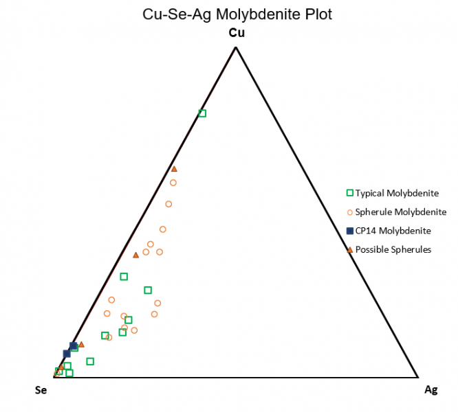
Figure 6.9 compares relative trace concentrations of Cu-Se-Ag. The plot shows a preference for selenium within typical molybdenite grains while spherical molybdenite realatively favor copper.
Figure 6.10: Fe-Se-Ag
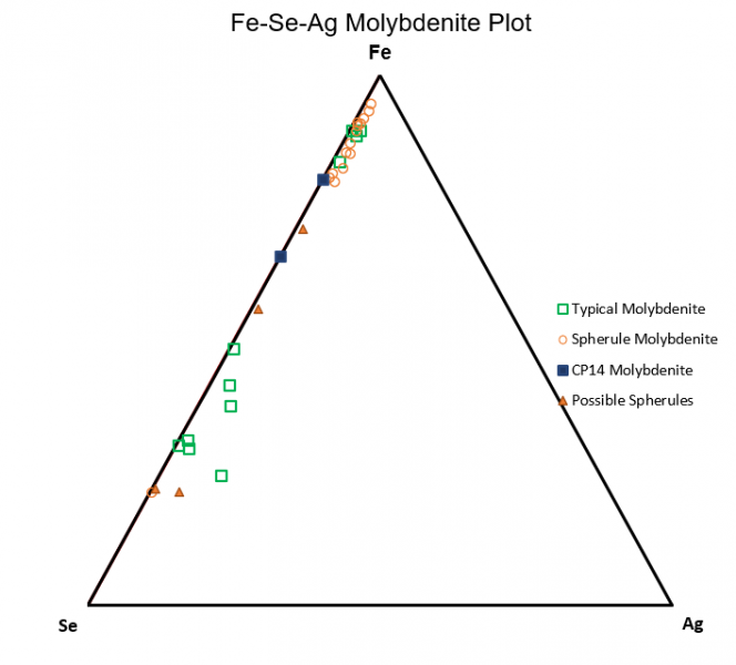
Figure 6.10 shows a comparison between some of the higher concentration trace elements. In the plot, it can be seen that spherical molybdenite has a strong preference for iron relative selenium or silver, while selenium alongside sulfur are more compatible relative to iron in typical molybdenite.
Results Summary
This triangle plots show some elements, relative to each other, are consistently more compatible in either typical or spherical molybdenite. This suggests a different formational environment, either geochemically, spatially, or both when each molybdenite type formed. The trace element results and relative compatibilities shown by these triangle plots can lend key information in better understanding the formational environment and conditions of each type of molybdenite and takes one step closer as to solving the enigma of Cave Peaks unique spherical molybdenite.
Discussion of hopes for Re/Os Dating
Our primary goal for this project has always been the analysis of the trace elements of the two different molybdenite habits found at Cave Peak and how they may possibly compare with each other. However, going into this project we had a secondary goal of looking at Re/Os dating to determine an age of formation for these samples; something that was previously attempted by other people but never achieved to a certain degree. Of course, in order to achieve this meant that we needed to get concentration values of Rhenium and Osmium from our scans of the grains. This was not the case. Looking through our data on iolite we found that there was essentially no Osmium in the samples as well as barely any Rhenium (average of 0.74 ppm across all molybdenite samples). These low and almost nonexistent concentrations made it obvious to us that we were not going to be able to do Re/Os dating. In addition, from these results we are able to understand why previous attempts are dating the Cave Peak molybdenite deposits failed.
Issues with OREAS-460-NP Standard
For this project with decided to use three standards. Those being: STDGL3, OREAS-460-NP, and GSE-1G. We chose these three due to their elemental compositions matching what we thought was going to be useful for our trace element analysis. A previous version of of the STDGL3, STGL2b2, was used in Ciobanu et al. (2012). When deciding on our standards we wanted to match them as much as possible to this. We ended up choosing OREAS-460-NP, however, once we ran our data through iolite and excel we found that this standard had too low recoveries. We chose not to use any of the data associated with this and rely only on STDGl3 and GSE-1G for our results.
Issues During Ablation
The biggest issue that arose while working on this project came as a surprise. Once we were able to sit down and start our data gathering with the LA-ICP-MS, during the pre-ablation process we saw that the counts coming in were dropping off extremely quickly and were basically unusable at that state. We quickly realized that the problem was that the laser was destroying our grains while it was doing its spots scans. This is because sulfides ablate very easily and very fast. The beam was too concentrated on those singular pre-ablation spots that even the setting the machine was at were too strong. This was especially true for the grains that were on thin sections. In our attempts to fix this we tried decreasing the laser power from 4.55 to 1.60 J/cm2 but that had little change on the destruction of our molybdenite grains. We attempted to remedy this issue by decreasing the repetition rate from 20 down to 5 Hz but by doing so we saw that the counts coming from the pre-ablation testing began pulsating.

This problem was quickly becoming a real issue since most of our samples at that point were spot scans. This coupled with the limited time we had in the lab to actually run these scans before going on Thanksgiving break made for a very stressful half hour of trial an error trying to figure out how to properly gather our data. In the end we decided on switching our method from being mostly individual spot scans to being only line scans across the various grains. This helped the grains actually survive the laser beam since it was no longer being focused on a single spot on the grains.