Methodology

Sample Preparation

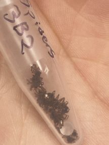
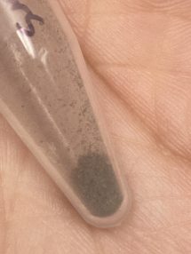
Figure 1. A sample before (top) and after (bottom) homogenization using a laboratory mixer

Arthropods were collected from Utqiagvik/Barrow, AK in late June through early July of 2025 using a combination of dry pitfall traps to capture terrestrial arthropods and an insect vacuum to capture aerial arthropods. Arthropods were identified and sorted by taxon, mostly to the family level. Arthropods were stored in a -20°C freezer before being dried in a Harvest Right freeze dryer for 24 hours. Three samples representing each taxon were selected for elemental analysis, usually consisting of multiple individuals to reach sufficient dry biomass for analysis. Samples were homogenized using a laboratory mixer in plastic centrifuge tubes with a silica ball bearing.

Figure 2. Samples before (top) and after (bottom) completing digestion in HNO₃ and H₂O₂

Samples were digested in an optima grade solution of 1 mL concentrated HNO₃ and 1 mL H₂O₂ in trace metal grade Savillex beakers on a hot plate at 120°C for 24 hours. After digestion, samples were dried on a hot plate before being dissolved in 1mL of 6M HNO₃. To arrive at a matrix of 5% HNO₃, samples were further diluted by a factor of at least 7.6 using Ultra Pure water. Based on relatively small sample dry masses and the known concentrations of analytes present in arthropod reference materials (KRIK-1, BFLY-1, and VORM-1), no dilution further than 7.6 times was determined to be necessary.

Analysis

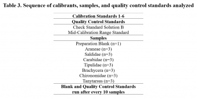
Solution-based ICP-MS analysis was conducted on seven arthropod taxa to determine their concentrations of cations B, Na, Mg, Al, P, K, Ca, Ti, V, Cr, Mn, Fe, Co, Ni, Cu, Zn, As, Se, Sr, Mo, Cd, Ba, and Pb using an Agilent 8900 ICP-QQQ at the University of Texas at Austin Department of Geological Sciences. The analytical method includes the use of an octopol reaction system (ORS) operated in helium (collision-mode) and hydrogen (reaction-mode) for removal of polyatomic interferences. Internal standards, mixed into samples via in-run pumping, were used to compensate for instrumental drift. Dilutions of stocks used to make a calibration curve were determined based on the maximum known concentrations of each analyte present in arthropod reference materials (KRIK-1, BFLY-1, and VORM-1). Blanks and standards used for calibration and quality control were prepared using trace metal grade reagents in acid-cleaned labware to have a consistent matrix of 5% HNO₃.

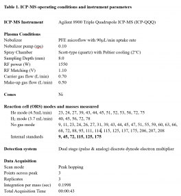
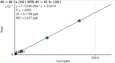
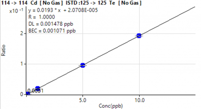
Figure 3. Representative calibration curves for a major element (Ca) and a trace element (Cd).

Calibration curves typically had a correlation coefficient of 1.0000 (Figure 1). Though the observed concentrations for many major elements were above the calibration curve, the extremely high correlation coefficients increase the likelihood that quantified concentrations are representative of the true concentrations in the sample.

For each analyte, the optimal mode of detection (Table 1) was selected by considering which mode yielded quality control standard recoveries closest to 1 and lowest relative standard deviation. Analyte recoveries obtained for two independent quality control standards were typically within 96.25-103.75% of certified values for analytes measured in optimal modes (Table 2). Limits of detection, based upon the population of blank (5% HNO₃) analyses interspersed throughout the analytical sequence were typically better than 0.38 ppb for analytes measured in optimal modes (with or without the ORS) (Table 2). The full procedural blank contained less than 0.061 ppb of most analytes, with P and K being the most concentrated contaminants at 5.735 and 3.396 ppb, respectively.

Statistical Analyses

One way ANOVAs were run for each analyte to determine whether arthropod samples varied in their analyte concentrations according to their taxon. Individual samples were mapped onto a PCA Biplot to visualize the contribution and correlation of analyte concentrations and resulting grouping (or lack thereof) of taxa and samples within taxa.