Methodology

Sample Collection

Samples were collected from the UT BEG repository of cores. The samples come from a core taken from Mirasol Springs that was collected via air rotary drilling. Five samples were selected to be analyzed, one from each geologic unit of interest: the Lower Glen Rose Limestone, Hensel Sand, Cow Creek Limestone, Hammett’s Shale, and Sycamore Sand.

Rock Digestion/Preparation for Analysis

All five samples were powdered by hand using an agate mortor and pestle. The powders were then digested using two separate methods: one to isolate just the carbonate fraction of each rock, and the other to dissolve the whole rock.

Carbonate Fractionation

Small centrifuge tubes (2mL) were weighed. About 100mg of sample was added to the tubes and weighed.

Using a pipette, 1.5mL of 0.2M NH4OAC were added to the tube. The mixture was hand shaken to fully expose the solid to the solution. After waiting five minutes, the samples were centrifuged for 5 minutes, which separated the liquid fraction from the solid fraction. The liquid fraction was decanted with a pipette. This process was repeated two more times using 1.5mL 0.2M NH4OACH, and then two times using 1.5mL ultrapure (“D2”) water, for a total of 3 acid washes followed by 2 water washes. When doing the water washes, the samples did not sit for 5 minutes before being centrifuged.

To dissolve the carbonate fraction, 1.5mL of 4% acetic acid were added to the tubes. The tubes were shaken to fully react the sample with the solute, and the tubes were left to react for 10 minutes with the lids open. The samples were then centrifuged 5 minutes. The solutions were pipetted into labeled beakers, and 1mL of 6N HNO3 was added to the sample. The samples were left on a hot plate over night to dry.

The following day, 200-300uL of concentrated HNO3 was added to each sample, and they were left to dissolve and dry. The following day, 0.5mL of 7M HNO3 and 0.5mL of ultrapure water were added to the samples.

Whole Rock Dissolution

Microwave digestion tubes were weighed. About 100mg of sample was added to the tubes and weighed.

About 5mL of HF and about 1mL of HNO3 was added to the samples. They were then run through a microwave digestor for an hour and a half. The samples were then added to labeled teflon beakers. The samples were dried and brought up in acid until all of the sample was dissolved. Then, the sample was finally dried again and dissolved in 0.5mL of 7M HNO3 and 0.5mL of ultrapure water.

Final Dilution

Once all of the samples were dissolved, the TDS of each sample was calculated and a dilution factor was determined. Each sample had to be diluted to a different extent. They were all diluted using 2% HNO3.

ICPMS Analysis

The samples and standards were ordered in the rack to run in the following order: calibration standards, quality control standard, single element standards, digested rock samples, quality control standard. Blanks were analyzed between each step.

To set up the run, all of the isotopes of interest were selected to be run, and the internal standards were delineated in the program. The concentrations of the standard solutions were entered as well. The instrument was then tuned using two methods: one that would cause low oxide production, and another that would cause high oxide production. Low oxide production was achieved by lowering the carrier gas rate to decrease the ratio of 140Ce16O/140Ce to about 1%. The high oxide production tune increased the oxide production ratio to about 3.8% by increasing the carrier gas rate. For each tuning, the CRC was run on no gas mode. Also, the omega lends was adjusted to be higher, which allowed higher isotope masses (REEs) to have preferentially higher counts than lower isotope masses.

Data Reduction

The data was given in counts/second, which was converted to a concentration in ppm through a series of steps. First, the data was corrected for drift using the concentrations of the internal standards. Then, the isotopic concentrations in the initial blank were subtracted by all of the following concentrations to correct for error.

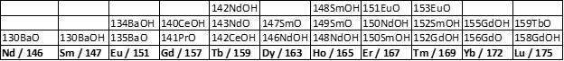
Then, the oxide production factors were calculated for the isotopes in table 1. To do so, the single element concentration of an oxide was divided by the concentration of the single element itself. The oxide production factors were multiplied by the REE concentration of the isotope that they mimic, and then subtracted by that REE.

Next, the equation of a line and regression were calculated using the counts/second of the calibration standards. Using the slope and y-intercept of the calibration curve, along with the counts/second of each isotope for each sample, the isotopic concentrations of each analyte could be determined. Next, the level of detection was determined for each isotope by multiplying the standard deviation of all of the blanks by the tinv of the blanks. The final isotopic concentrations for each rock sample were calculated by multiplying the dilution factor by the concentration, and converting to ppm by dividing by 1000.