Proposal

Abstract

The objective of this method project is to determine the optimal operating conditions and quantification limit for ultra-trace zinc concentrations and arsenic concentrations in urban stream waters. In previous analysis of natural waters in Austin by the Banner research group, we have seen concentrations of Zinc as high as 250 ppb, but concentrations on average in Austin and utilized by other researchers have been around 2-5 ppb (Christian et al., 2011, Garnier et al., 2024, Le Pape et al., 2012). Arsenic concentrations have been utilized below 1 ppb by other researchers (Garnier et al., 2024), and concentrations in the Austin watershed have shown to be as high as 6 ppb based on historic Banner research group Austin measurements, but the average sits around 1.2 ppb. At the end of this project we will define the quantification limit for zinc and arsenic concentrations when both are calibrated up to 25 ppb. The most frequent measurements from our own lab results (CRESSLE) are in this range, and we want to know the lowest values that can be quantified and still differentiated from the background, and therefore quantify uncertainty at low concentrations for zinc and arsenic on the ICP-MS. The concentration of zinc may be used to inform the running of samples with TIMS or MC-ICP-MS, such as indicating the need for and extent of preconcentration. The isotopic ratios determined by TIMS or MC-ICP-MS will play an important role in research related to Project CRESSLE, which is an interdisciplinary research project focusing broadly on water quality and urbanization in underserved areas of Austin.

---

Research Objective and Specific Method Objectives

---

Justification

This method is of potential importance because we are specifically interested in low level zinc and arsenic concentrations in water. Some previous zinc results from natural waters have had large analytical uncertainties because the measured concentrations were so low. Optimizing the sample collection and preparation along with the ICP-MS method for zinc at low concentrations would help solve some of these problems. Because natural concentrations of zinc and arsenic are so low, often below 25 ppb for Zn and below 10 ppb for As, it is difficult to make a comparison between urban and rural environments for these systems. We are interested in getting high precision and accuracy because we want to measure very low concentrations of zinc, but because zinc has a high first ionization potential, it is harder to produce a strong signal comparable to background noise. Finding ways to combat this issue with precise methodology will allow us to proceed with research into pollutant tracing with zinc and overall water quality research.

---

Review of Relevant Work

Previous studies have successfully determined the source of zinc in natural waters (Tu et al., 2020) and have even observed daily changes in zinc concentrations, using ICP-MS, which were accredited to urbanization (Froger et al., 2020). Additionally, the use of zinc isotopes and associated zinc concentration data is emerging as a potential tracer for urbanization in watersheds (Desaulty et al., 2020a, Desaulty et al., 2020b, Garnier et al., 2024, Rosca et al., 2019, Tu et al., 2020). Some of these have included zinc concentrations less than 5 ppb. Specifically, Le Pape et al. studied urbanization in a watershed and drew conclusions using zinc concentration data that was all less than 10 ppb. Trace elements were measured using ICP-MS with a collision gas that was 7% H2 and 93% He for both zinc and arsenic (Le Pape et al. 2012). This paper did not see an increase in arsenic concentrations with urbanization. Low concentrations of zinc are still important to be able to resolve because low concentrations can have small but measurable changes in zinc isotope ratios (Desaulty et al., 2020b).

We are also interested in measuring arsenic and quantifying arsenic uncertainty at low concentrations. Arsenic is a heavy metal that is dangerous for public health and is also related to urbanization and urban industries such as semiconductor use (Alexakis et al., 2021, Li et al., 2021, Martinez-Morata et al. 2022). Past studies have measured arsenic concentrations by county in order to compare concentrations to EPA updated standards and were able to differentiate concentrations below 5 ppb as they related to socioeconomic factors (Nigra et al., 2020). Others have consistently measured 1 ppb spikes using ICP-MS helium collision mode in the CRC, showing the potential for low concentration, yet still significant measurements (McCurdy).The FDA, however, has reported the limit of quantification for arsenic using ICPMS on food or food related products to be over 11 ppb while the LOD is 1.27 ppb (Elemental Analysis Manual (EAM), 2022). This warrants additional research into our limit of quantification as it relates to our LOD. 

---

Materials and Methods

A likely analytical challenge will be ensuring there is no contamination in our samples. Because of how common Zinc is, contamination is possible. To do our best to track this, we will monitor with blanks as frequently as possible.

Developing and Testing the Method

We plan to start our method development by using experimental conditions from recent papers (Desaulty et al., 2020, Alhagri et al., 2024, Froger et al., 2020, Tu et al. 2020). Multiple papers reported using In and Re as internal standards and using NIST SRM 1640 as a standard (Desaulty et al,. 2020, Fruger et al. 2020, Tu et al. 2020). We will use Inorganic Ventures IV-68017 as our standard for Zn, which has 100ppm zinc and we will reference as A1, and Inorganic Ventures MSAS-10PPM as our standard for As, which has 10 ppm arsenic and which we will reference as A4. For our QC standards, we will use the same standard types from the same manufacturer, but a different lot number, which will be referenced as QCBL4. Our calibration standards will be of low concentration to optimize our statistics and minimize carryover. Accuracy and precision will be determined by creating calibration standards over a range of low concentrations, analyzing replicates of samples, and using internal standards. We will test our method by running calibration or QC standards as unknowns and comparing the results to the known values.

This project is focused more on constraining instrumental uncertainty at low zinc and arsenic concentrations rather than investigating laboratory and sample preparation practices that may lead to contamination. As such, we will take extra care to limit contamination during sample preparation by using acid-cleaned teflon bottles for sample preparation and will handle samples the fewest amount of times possible to prevent zinc transfer from gloves, which is a  documented source of contamination (Garcon et. al, 2016).

Our method will use a lower calibration range for zinc compared to previous analyses. Other analyses calibrated up to 1,000 ppb, which could cause problems at low concentration levels depending on the goodness of fit of the calibration curve. We plan to calibrate only to 25 ppb for Zn and only up to 25 ppb for As which will hopefully give a better fit at lower concentrations. 

 We will determine the detection limit by making a series of spikes at increasing concentrations. We will then systematically run replicates of the spikes starting at the lowest concentration and assess if the signal is distinguishable from the background. This, combined with frequent blanks and increased rinse time to increase washout and prevent carryover, will ideally result in the highest accuracy and precision.

Interferences

A major interference for As-75 is ⁴⁰Ar³⁵Cl. This will not be a significant issue for our method because we plan to analyze samples using He as a collision gas. Zn-64 has an interference with ⁴⁰Ar²⁴Mg, but this will once again not be a significant issue because our samples will be analyzed using He as a collision gas. Zn-68 has interferences with doubly charged Barium and doubly charged Cerium, as well as argon interferences, but using a collision cell with helium gas should mitigate these effects.

Sample Set

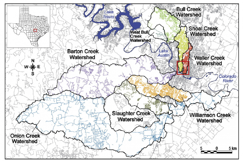
In the future we plan to analyze stream water samples from several watersheds in the Austin area. For this project, however, we plan to use blanks and standards as unknowns as well as field blanks to rule out sample prep as the source of variability. A sufficient number of samples will be analyzed to determine the detection limit of Zn and Cu. It’s hard to give a precise number for the sample set at this point, as it depends on the number of tests that will be required to determine the optimal method. We plan to analyze a minimum number of samples while considering accuracy and precision. A rough estimate at this point is 30-40 samples per test, including all calibrations, QCs, and blanks. 

A large portion of the sample set will be blanks. The majority of the blanks will be laboratory blanks composed of type I (18.2 MΩ-cm) water. Field blanks collected at sampling sites will also be analyzed. In order to determine the method detection limit, many lab blanks will be analyzed. A method detection limit (MDL) will be determined following the method of using replicate measurements of spiked blanks in 40 CFR 136. In this method, a sufficient number of blanks (>7) are analyzed to get an estimate of the background concentration. The detection limit is then estimated based on the signal to noise ratio of the blank. Then blanks are spiked with a concentration of sample 2-10 times that of the estimated detection limit for both analytes and analyzed for a sufficient number of times. After the analyses the MDL is calculated, using a 99% confidence interval and student’s T test. Thus, more replicates will give greater confidence in the detection limit . The detection limit formula is as follows : 

MDL = t_{(n-1, 0.95)}S

Where t_{(n-1, 0.95)} is the Student’s t statistic value based on the number of replicates and S is the standard deviation of the replicate measurements (40 CFR 136).

We will also calculate a limit of quantification (LOQ), which is a more practical limit set as some multiplier above the MDL. The LOQ is the lowest concentration that can be measured with a required degree of certainty while the MDL is the lowest concentration that can be detected by the instrument. 

---

Possible Outcomes

Determining the limit of quantification will allow us to continue the analysis of zinc and arsenic in our research for Project CRESSLE with more confidence in the data. Because measurements are near the limit of detection, it is hard to distinguish significance values from background. By limiting carryover through blanks and increased washout time, lowering calibration standards to more realistic ranges for our waters, and running replicate spikes near the limit of quantification, we will ideally determine how low concentrations can be measured reliably, and what should be considered too low for analysis. 

It may also prevent future issues, and expenses, with not precise enough readings to find significance in trends. This will allow for the development of more robust, quicker, and less expensive research on using zinc as a tracer of anthropogenic sources. 

---

Timeframe and Budget

Based on our proposed sample set, we have a budget of $1440. This is realistic because optimizing methods for ultra-trace zinc and arsenic concentrations will help advance our research goals and allow for high quality data collection in the future. As for time, we plan to run our samples using the autosampler overnight and therefore will not be budgeting for time. 

Budget Breakdown: 

1st Run: 

• Pre-calibration blanks: 3
• Calibration Standards: 4
• Blanks:5
• QCs: 1
• Blanks for analysis: 7

2nd Run

• Pre-calibration blanks: 3
• Calibration Standards: 4
• Blanks:5
• QCs: 1
• Blanks: 5
• Spike 1 replicates: 7
• Blanks: 1
• QCs: 1
• Blanks: 1
• Spike 2 replicates: 7
• Blanks: 1
• QCs: 1
• Blanks: 5
• Spike 3 replicates: 7 
• Blanks: 1
• QCs: 1
• Blanks: 1