Results

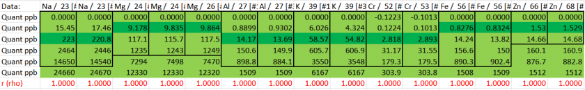
I evaluated how well the calibration range constrained the measured analyte concentrations and, based on this assessment, established concentration bracketing for the samples. This approach shows that the calibration curve effectively encompasses the range of analyte concentrations present in the samples, thereby improving the accuracy and reliability of the analysis.

Table 5: Concentration bracketing for the samples

Data Reduction

To identify the analyte modes that achieved optimal accuracy and precision, we evaluated their performance in terms of both sample analysis and quality control (QC) standards. Those analytes are highlighted in yellow in table 6.

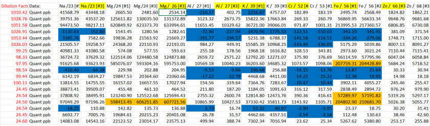
The actual concentrations in the samples are calculated by multiplying the measured values by their respective dilution factors. As indicated in Table 6, the 1000x dilution caused some analytes to fall below the detection limit, highlighted in blue, while the 100x and 25x dilutions resulted in certain analytes exceeding the upper limit of the calibration standard, shown in orange gold. This underscores the need for careful selection of dilution factors to ensure the analyte concentrations fall within the calibration range for accurate quantification.

Table 6: Adjusted analyte concentrations

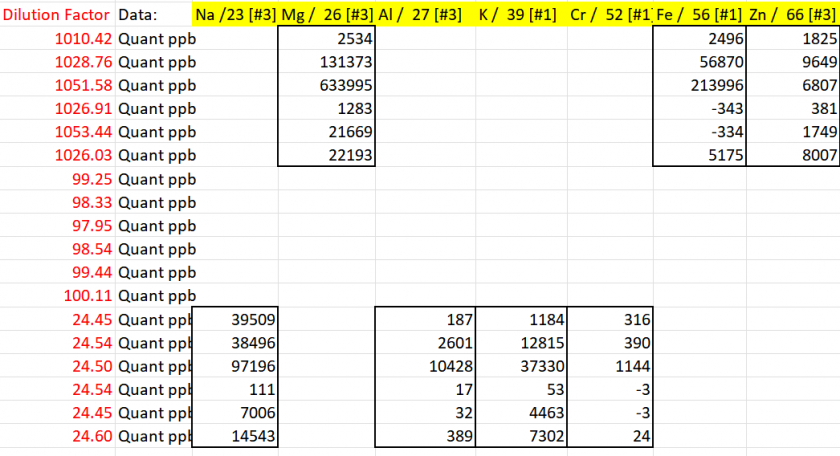
To create the final data table, we focused on including only the sample results obtained using the most effective analytical modes and the optimal dilution level. This ensures the highest accuracy and reliability of the data. The outcomes of this selection process are summarized in Table 7.

Table 7: Final Sample Results Based on Optimal Analytical Modes and Dilution Levels

The concentrations of the analytes are presented in Table 8, providing a comprehensive summary of the final calculated values based on the selected optimal analytical modes and dilution levels. This table highlights the precise quantification of each analyte in the samples.

Table 8: Final Concentrations of Analytes in Samples