Touring UTIG’s Airplane

April 29, 2016

By Laura Lindzey, a graduate student at the Jackson School of Geosciences. The post first appeared on her blog. 

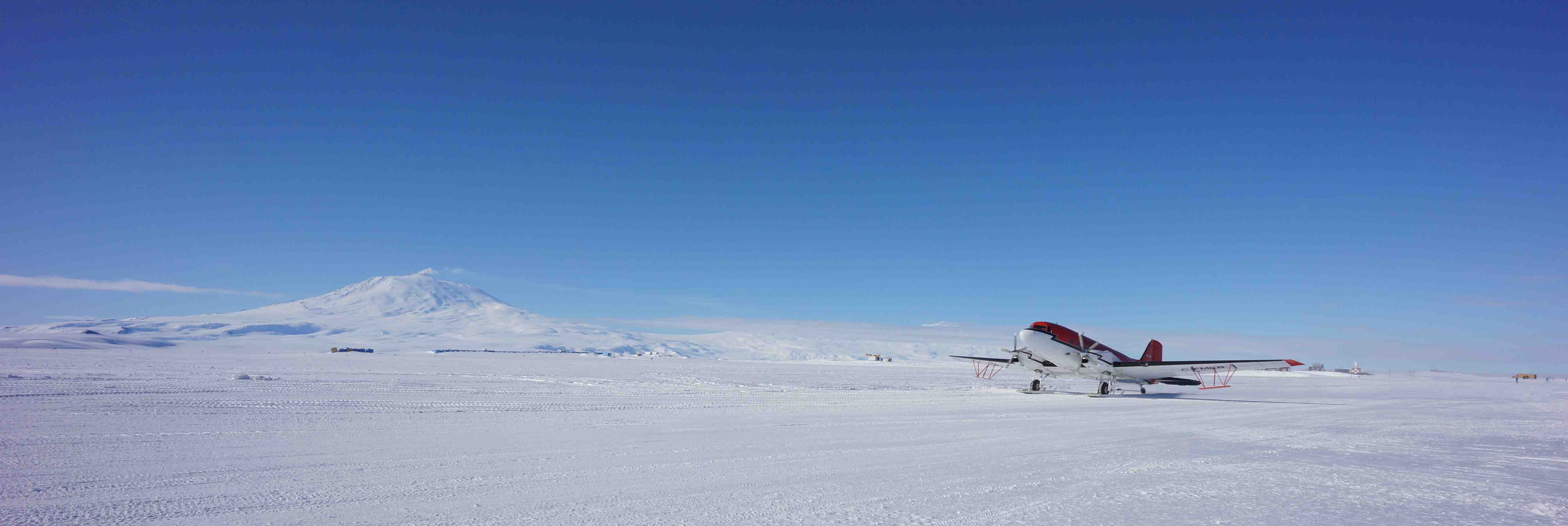
Don Blankenship’s research group at UTIG has been collecting geophysical data in Antarctica for decades. Each season, we hire Kenn Borek Air¹ to operate one of their modified airplanes, stuff it full of sensors, and fly around Antarctica. This post attempts to give a tour of the hardware involved, with an emphasis on its scientific purpose and a detour through Antarctic logistics.

Why aerogeophysics?

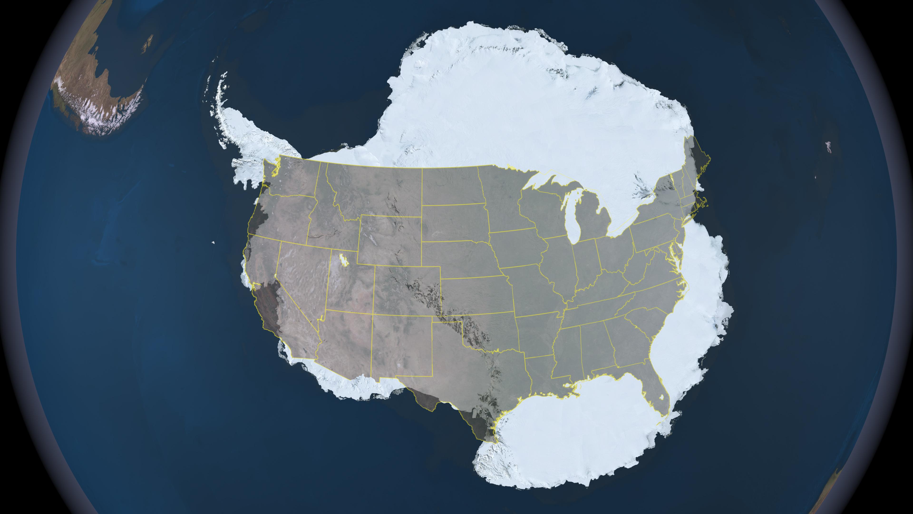Antarctica is huge and hard to access. While some types of data require in situ measurements the most efficient way to obtain basic information about the thickness of the ice and properties of the rock underneath it is to mount sensors in an airplane and start flying. This type of mapping is inherently 1D in nature – we obtain very dense observations along a flight line, then interpolate tens of kilometers between the lines to create a map.

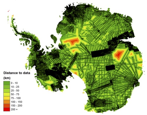
Black lines in the plot above show everwhere that BEDMAP2² has ice thickness data. Until this season, there were places where the closest airborne measurement was hundreds of kilometers away, and the ice thickness estimate is based on very low resolution satellite gravity measurements!³

The airplane (and logistics)

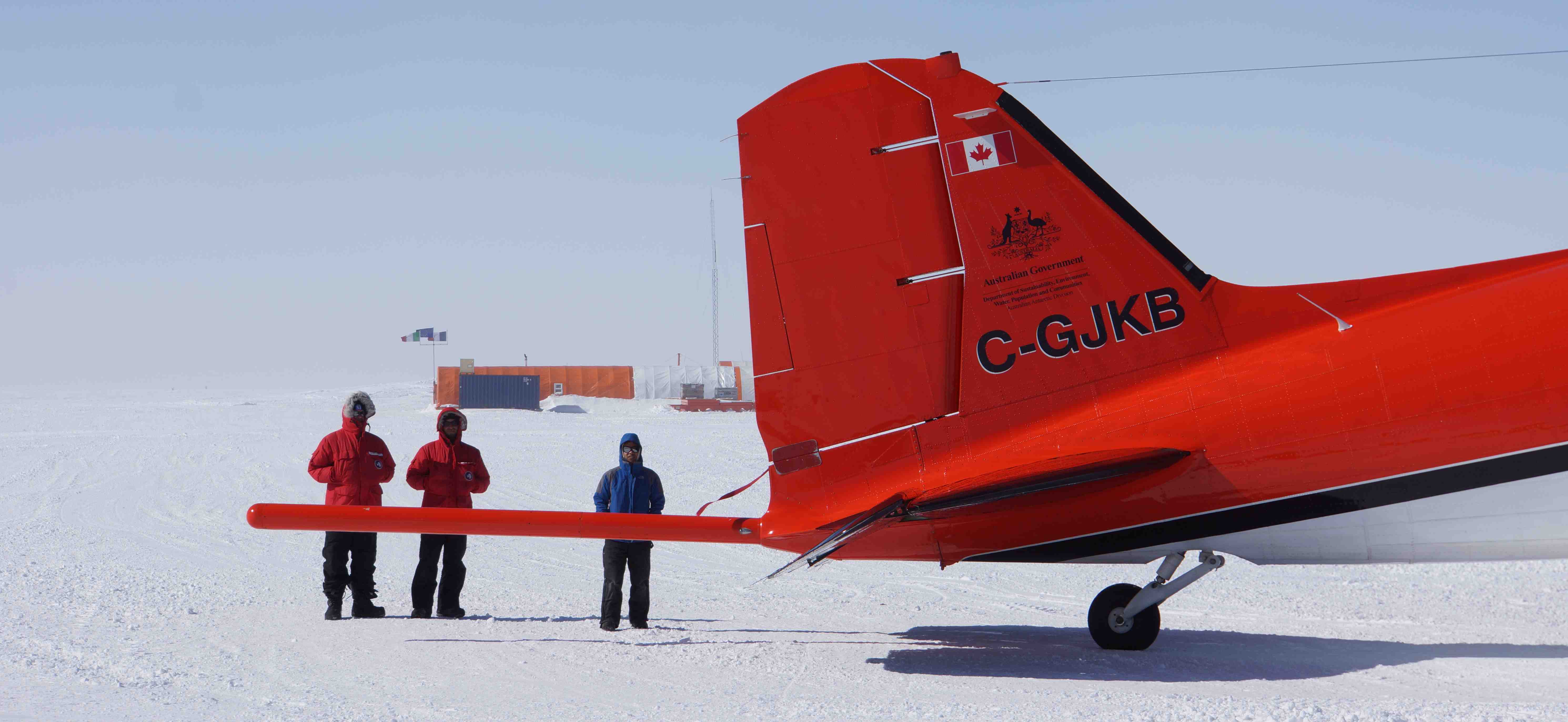
My research group currently uses WWII-era DC-3s,⁴ like the one in the picture at the start of this post.⁵ We’ve used these since 2007. All through the 1990’s and early 2000’s, they used a Twin Otter (below). Conceptually, not much has changed – while we’re continually upgrading the instruments, the same types of data have been being collected for over 20 years.

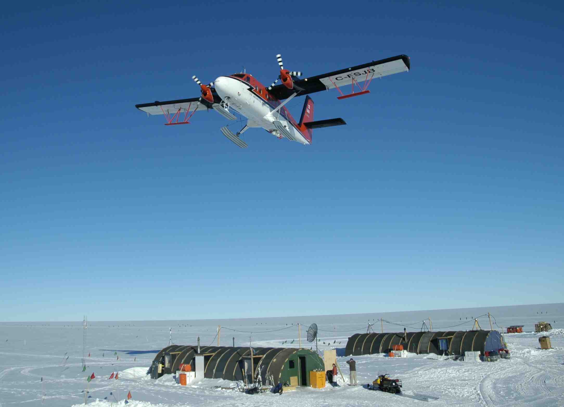
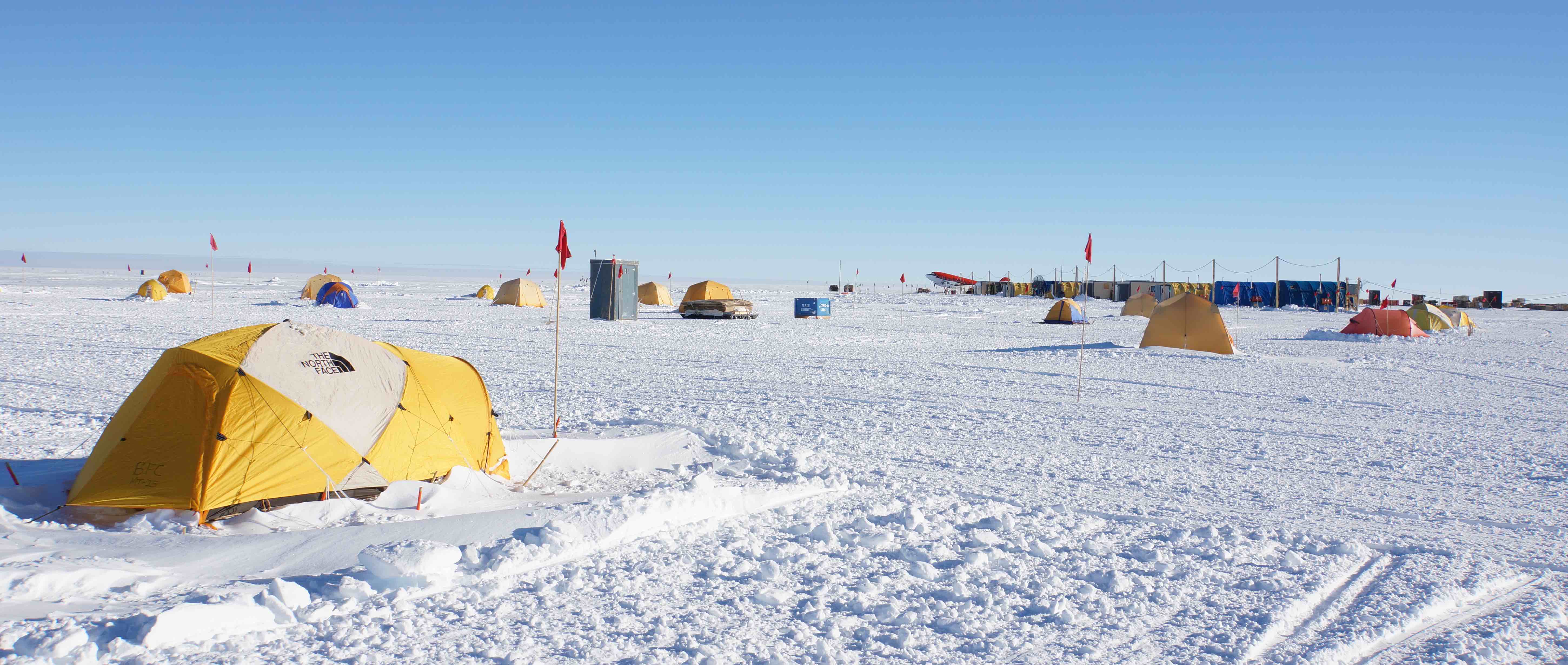
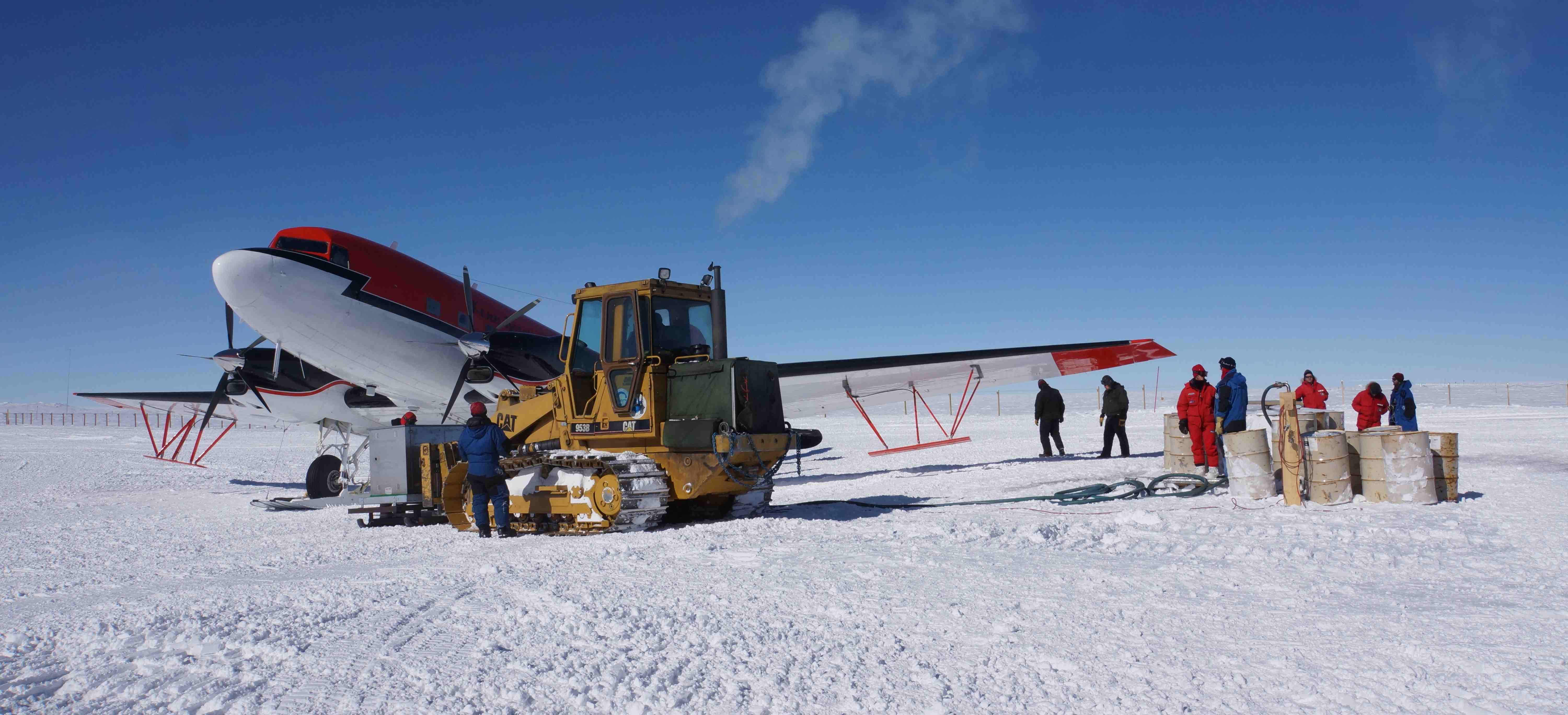
Each season is different, but a common pattern is to ship everything to a larger coastal station (McMurdo or Casey), where we install and test our instruments. We then fly from there to a base closer to our study area. This might be another station, a series of stations, or even a field camp. The image below is the WAIS Divide field camp, where I spent about a month last year – sleeping in a tent was surprisingly comfortable! We’ll stay anywhere from a few days to a month at each location, then transit back to the original station to pack up and head home.

I may have mentioned stuffing the airplane full:

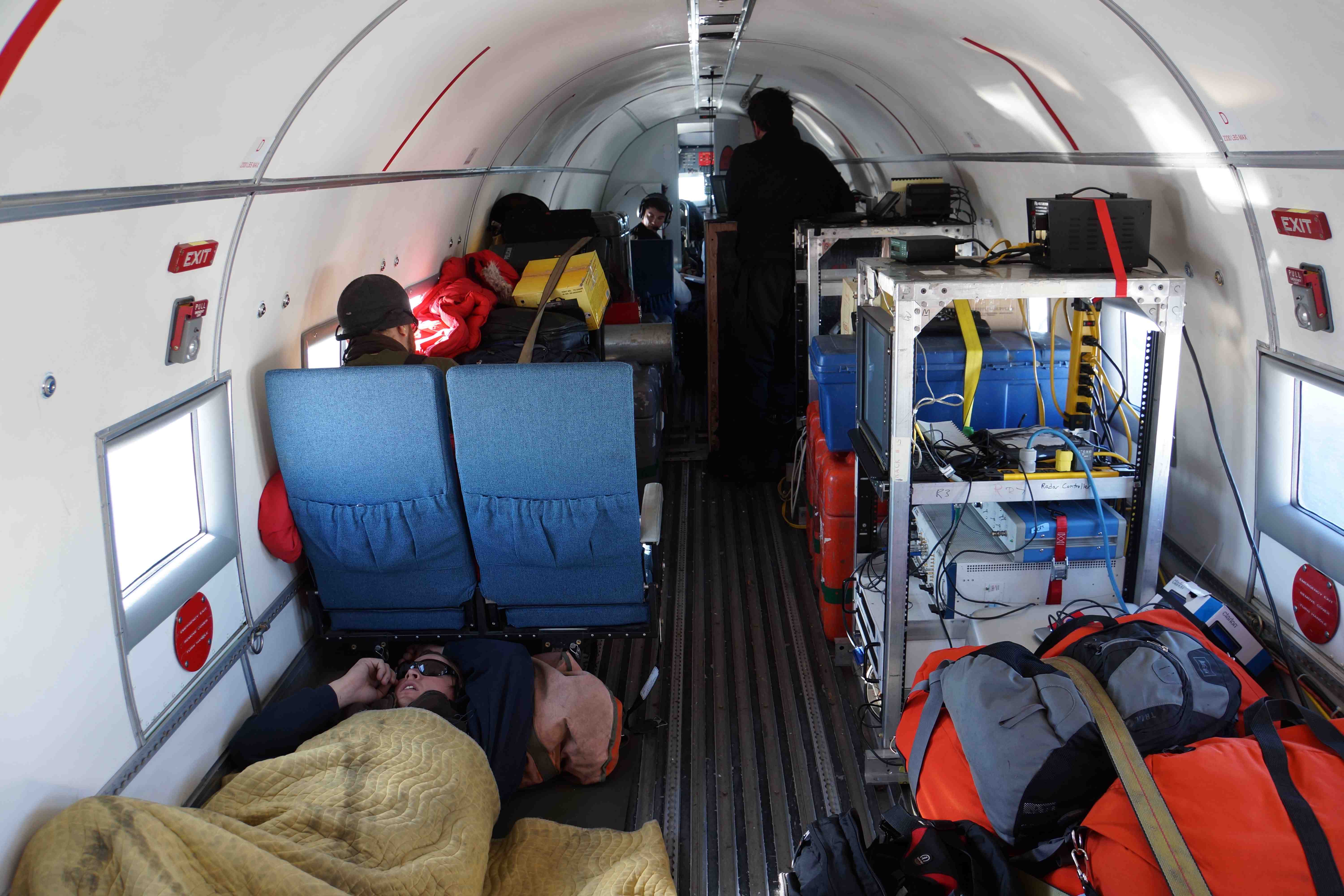
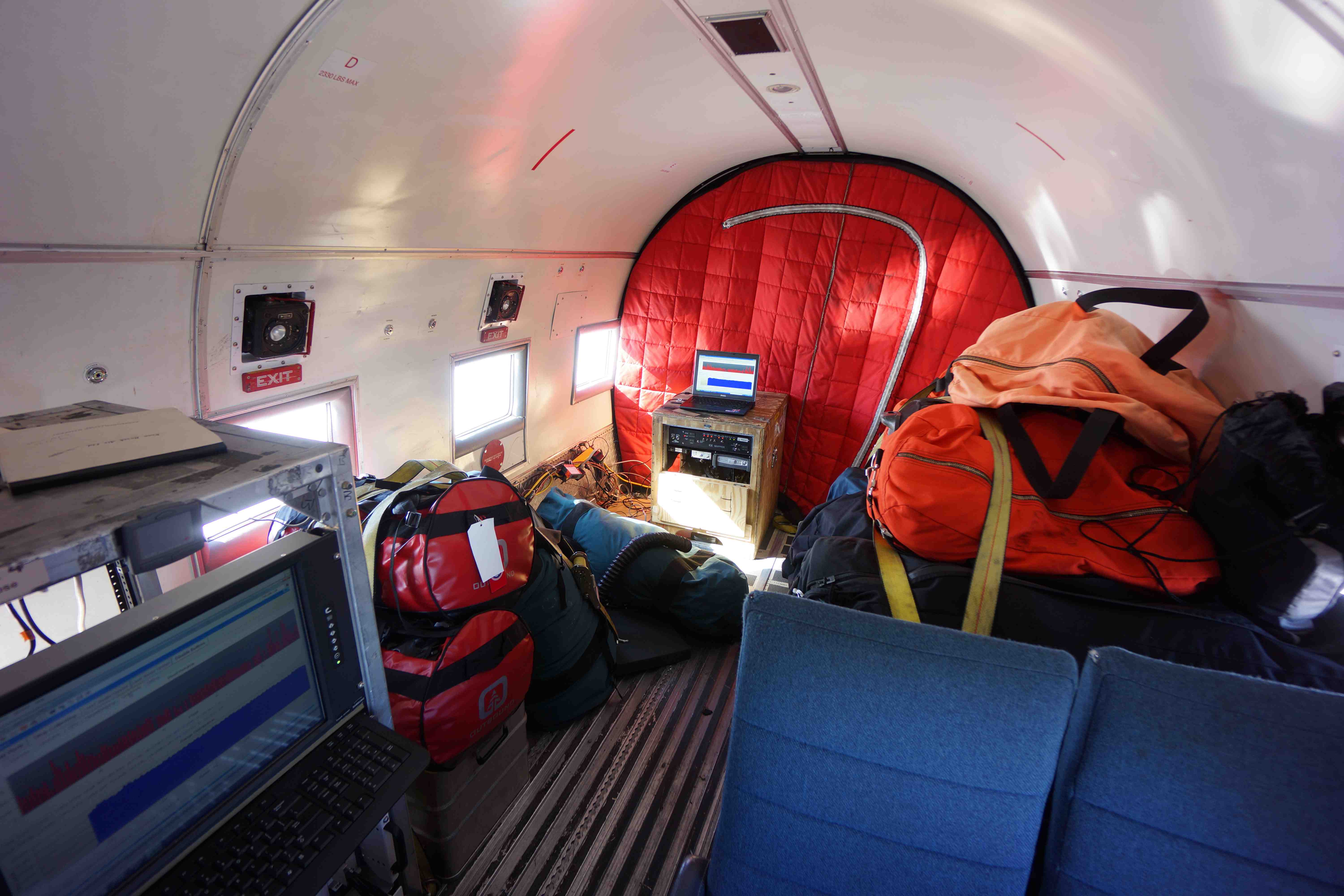
The above images are from transit flights, when we had way more people and baggage than for normal survey operations. The right photo was taken looking from the center of the plane towards the back. In it, we can see part of rack 4 (used for HF radar electronics), the photon counting lidar with its control laptop⁶ on top, and the curtain that separates the heated part of the plane from the cargo doors.

From a similar location but looking forward (and taken on a non-transit flight!) we get a nice look at the racks in the front half of the airplane:

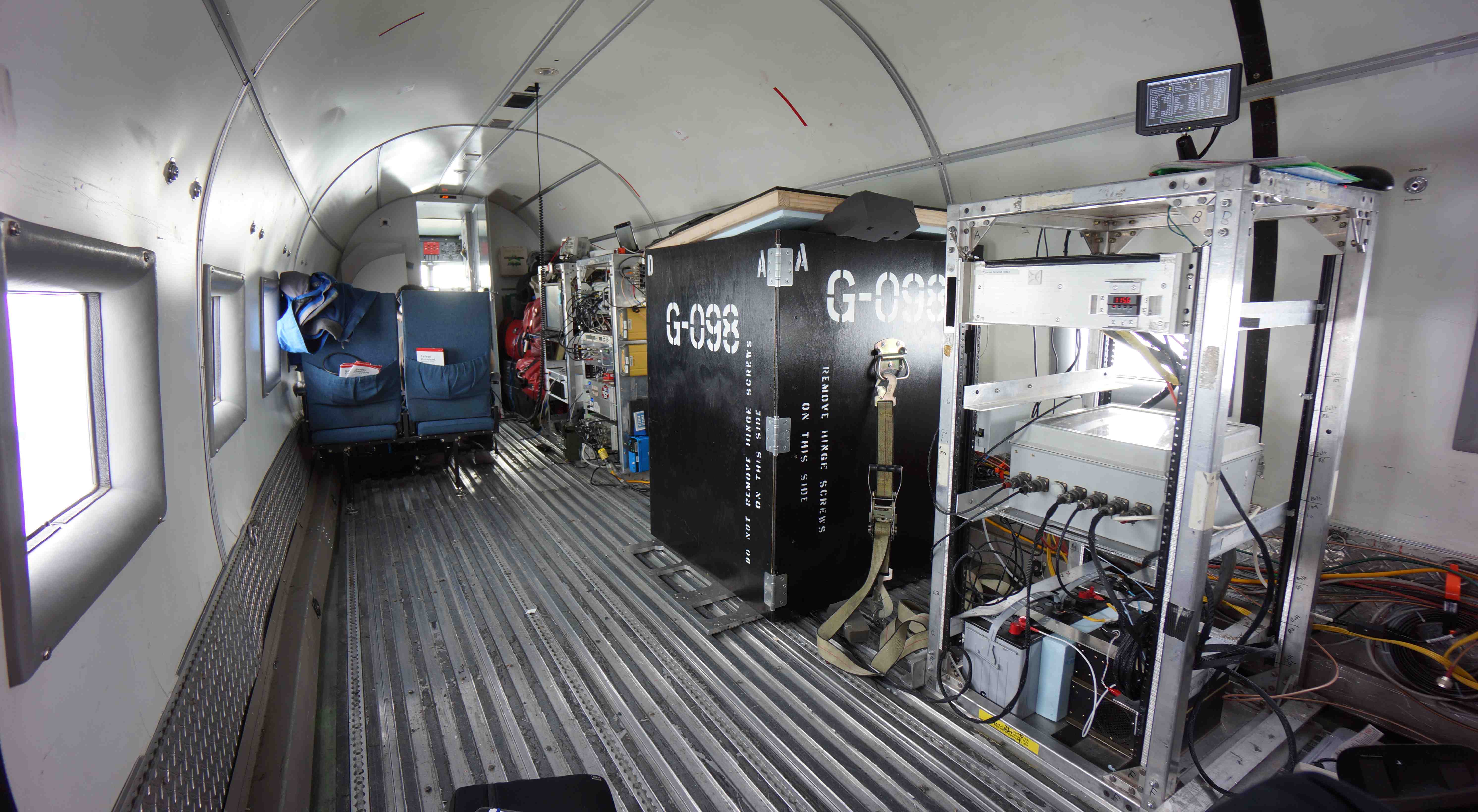
Starting at the cockpit, we have:

• rack 1 – operator interface, VHF amplifier
• rack 2 – VHF radar electronics
• black box – gravimeter
• rack 3 – gravimeter electronics

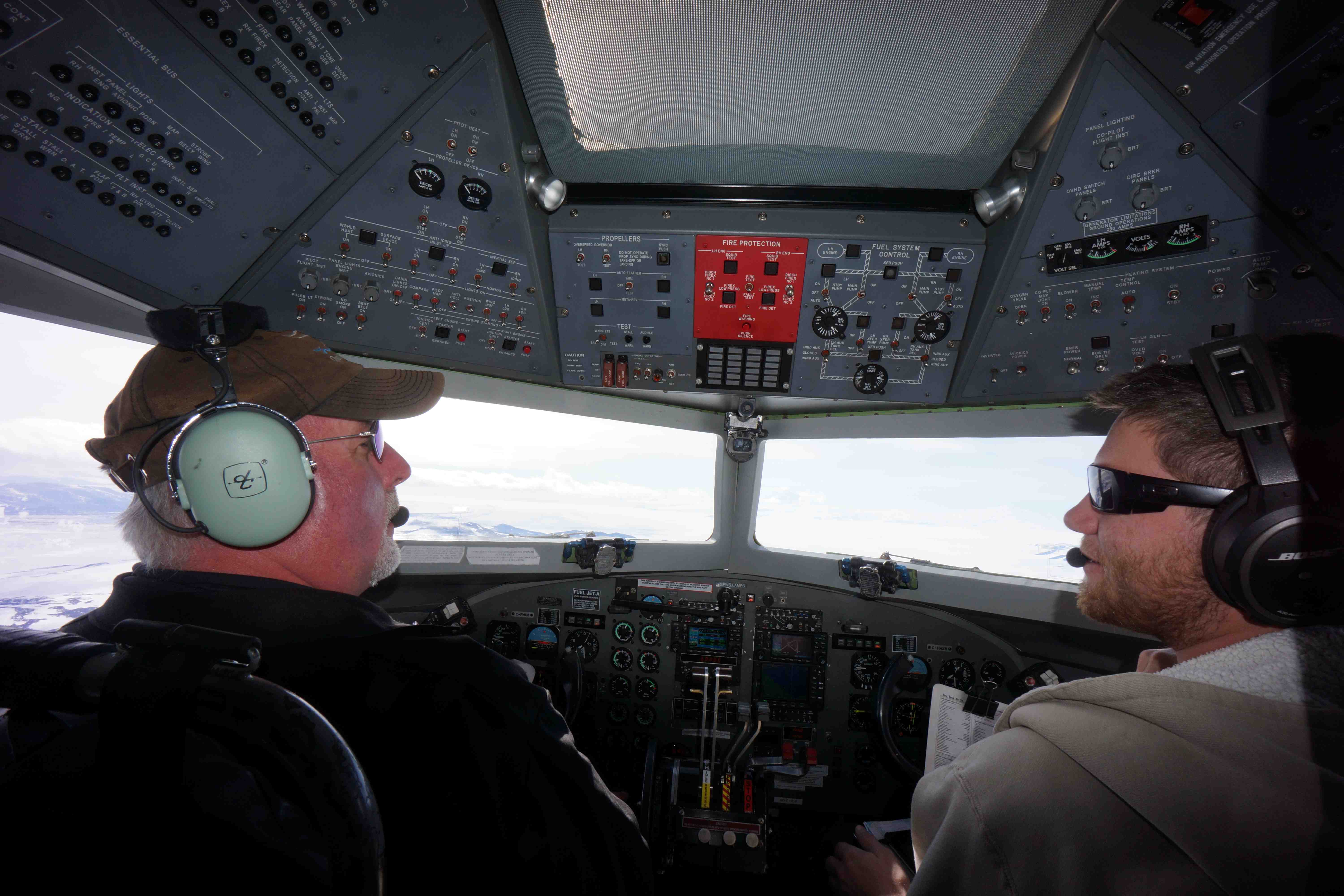
Any Kenn Borek airplane comes with 3 people dedicated to its operation: a mechanic (who is usually waiting back at the station), a pilot, and a copilot. Here are Kevin (left) and John (right), our pilots last season.

We find that the DC-3 has the best tradeoff for fuel burned per line-km of data collected.⁷ This airplane burns ~1000⁸ pounds per hour,⁹ travels at a nominal cruising speed of 160 knots, and has an endurance of ~6.5 hours in survey configuration.¹⁰ So, for every day of good weather, we can get up to 2000 line-km of data. If the weather has been bad and the pilots have extra hours available, we might do two 5-hour flights rather than a single 6.5 hour one, but that’s the maximum for a single flight crew.¹¹

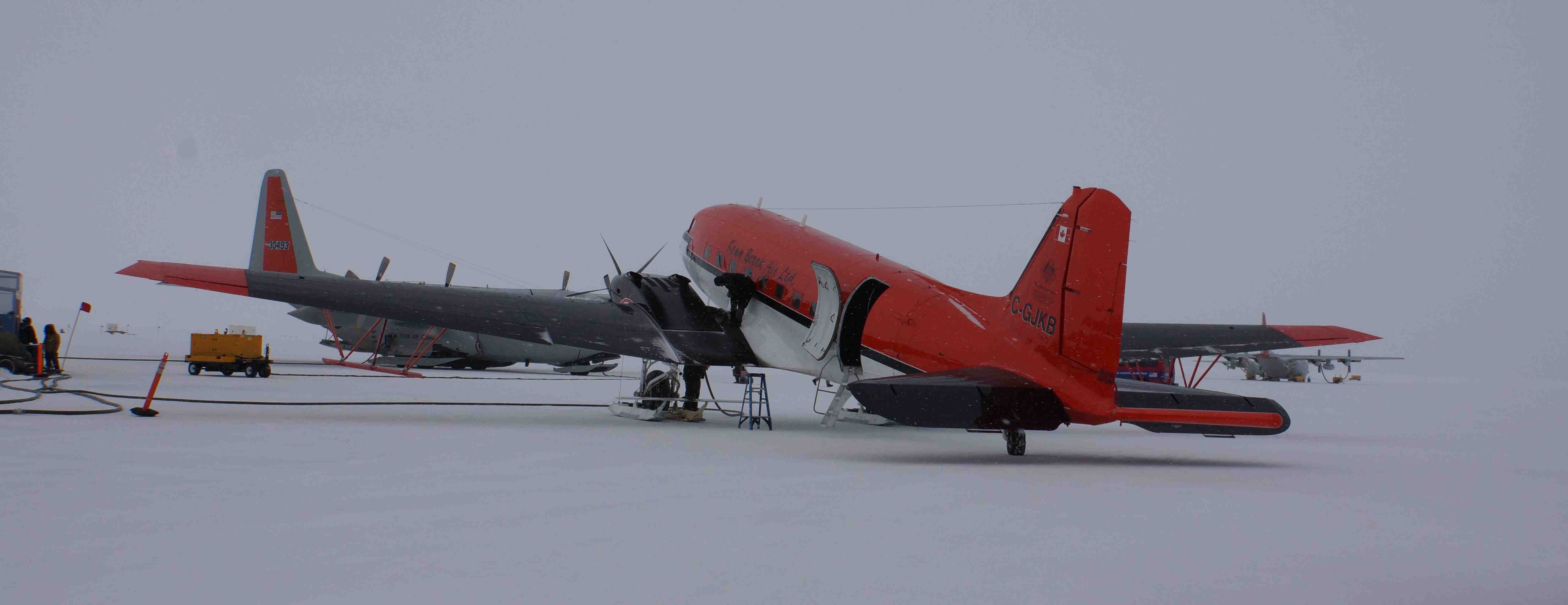
Antarctic weather is usually the biggest challenge to successfully flying all of the survey lines that we’ve planned. At a rough estimate, we’re only able to fly 1/2 of the days when the airplane is available. The biggest worry here is the ability to land. When you’re using snow for a runway, it doesn’t take much in the way of clouds or fog to ruin all contrast. Add a few more clouds or some snow falling from the sky as in the picture above, and it can be hard to find the horizon when you’re just walking around. Clouds are also a problem because of the potential for the wings – or worse, the radar antennas – to ice up. Where we were operating last season, there were no good alternative runways, which meant that we were only able to fly when the weather was forecast to be pristine for the next ~8 hours.¹²

Once we have everything installed and are airborne, what data are we collecting?

VHF Radar

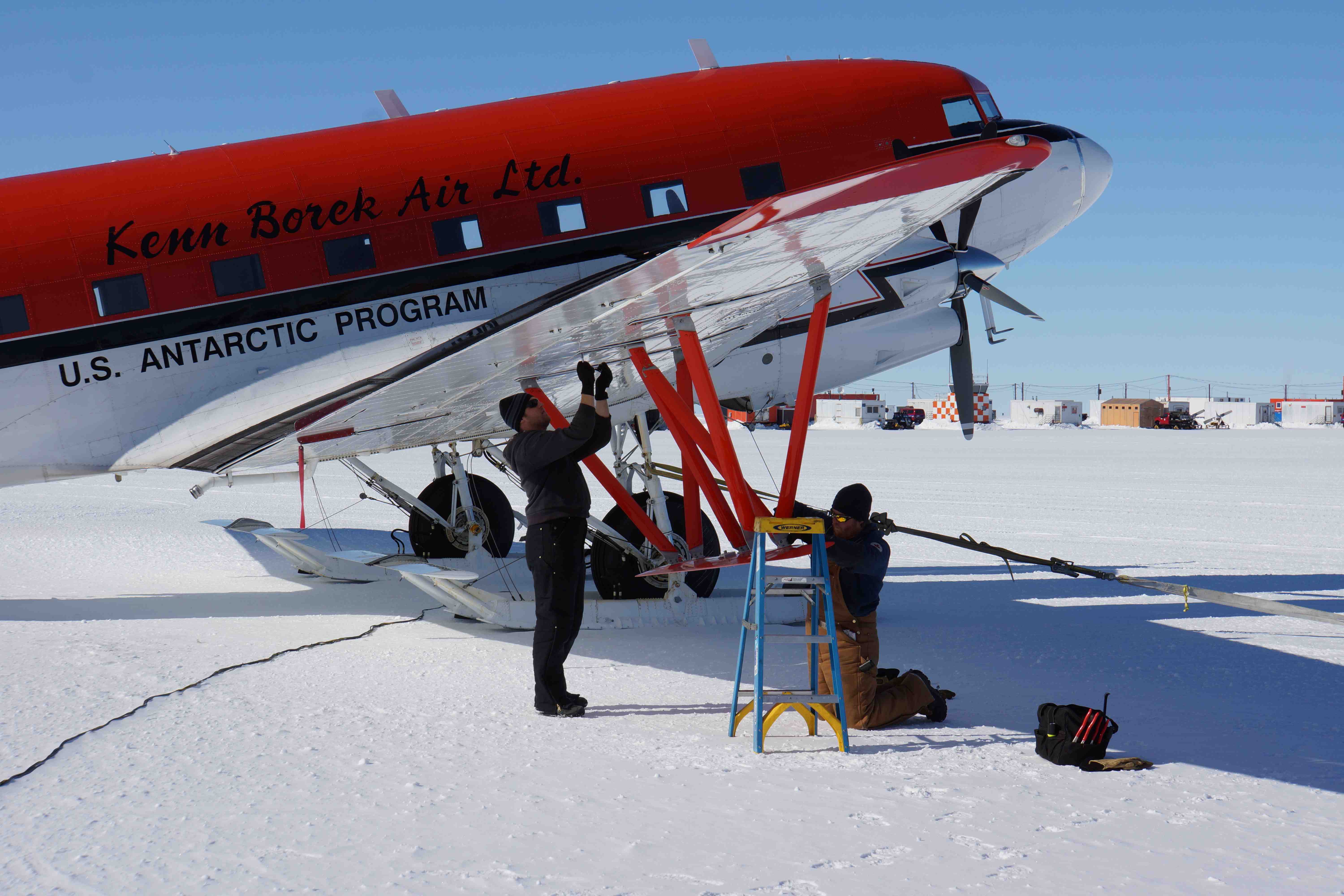
The most visible external modifications that we make to the airplane are the antennas installed under each wing for the 60MHz VHF radar that we use to get a 2D cross section of the ice. While the receiver electronics have changed multiple times since then, these antennas are the same ones that were used back in the 1970’s for some of the first ice-penetrating radar surveys of Antarctica.¹³ Both antennas are used both for transmitting the 8kW signal and for receiving the much weaker echoes.

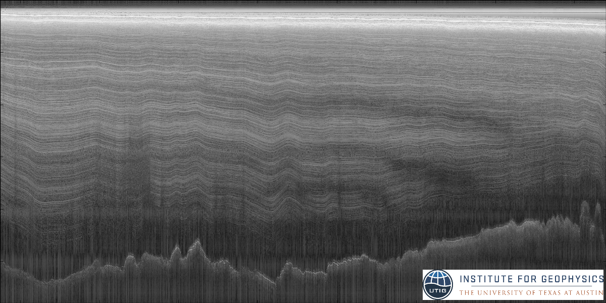
An example of the data is shown above – you can clearly see the ice surface, layers within the ice, and mountains underneath. I’ve previously talked about interpreting the radargrams, so I won’t go further into it here.

The most basic science done with data from this sensor is determining the topography underneath kilometers of ice. Among other things, this is important for calculating how much potential sea level change is locked up in Antarctica, and how stable the ice sheet is likely to be.

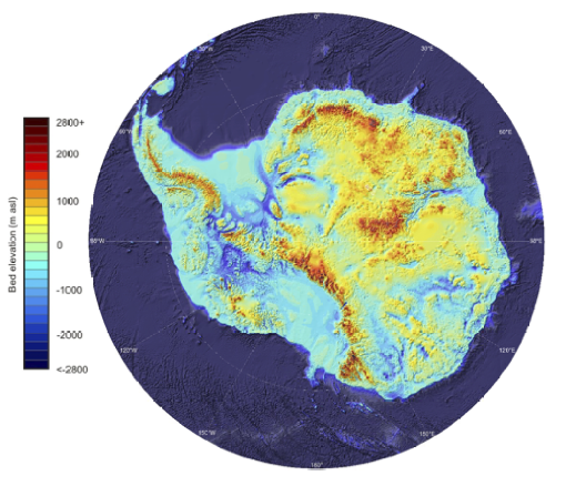
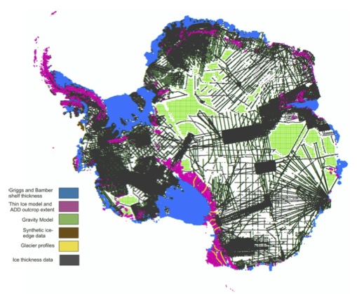
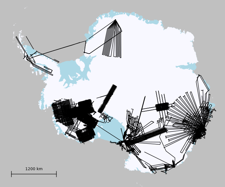
We are proud of having collected a significant portion of the line-km that were used to create Bedmap2.¹⁴ Bedmap2¹⁵ is the most recent compilation of Antarctic ice-depth and sub-ice topography data.¹⁶ The large image above shows the bed elevation – note how much of the continent is actually lower than sea level! The smaller image on the left shows the source of the data. Almost all of the black lines represent a single flight line. The densest (apparently solid) regions of black lines correspond to grids with 5km line spacing. The right plot shows where my research group has flown over the past few decades.

HF radar

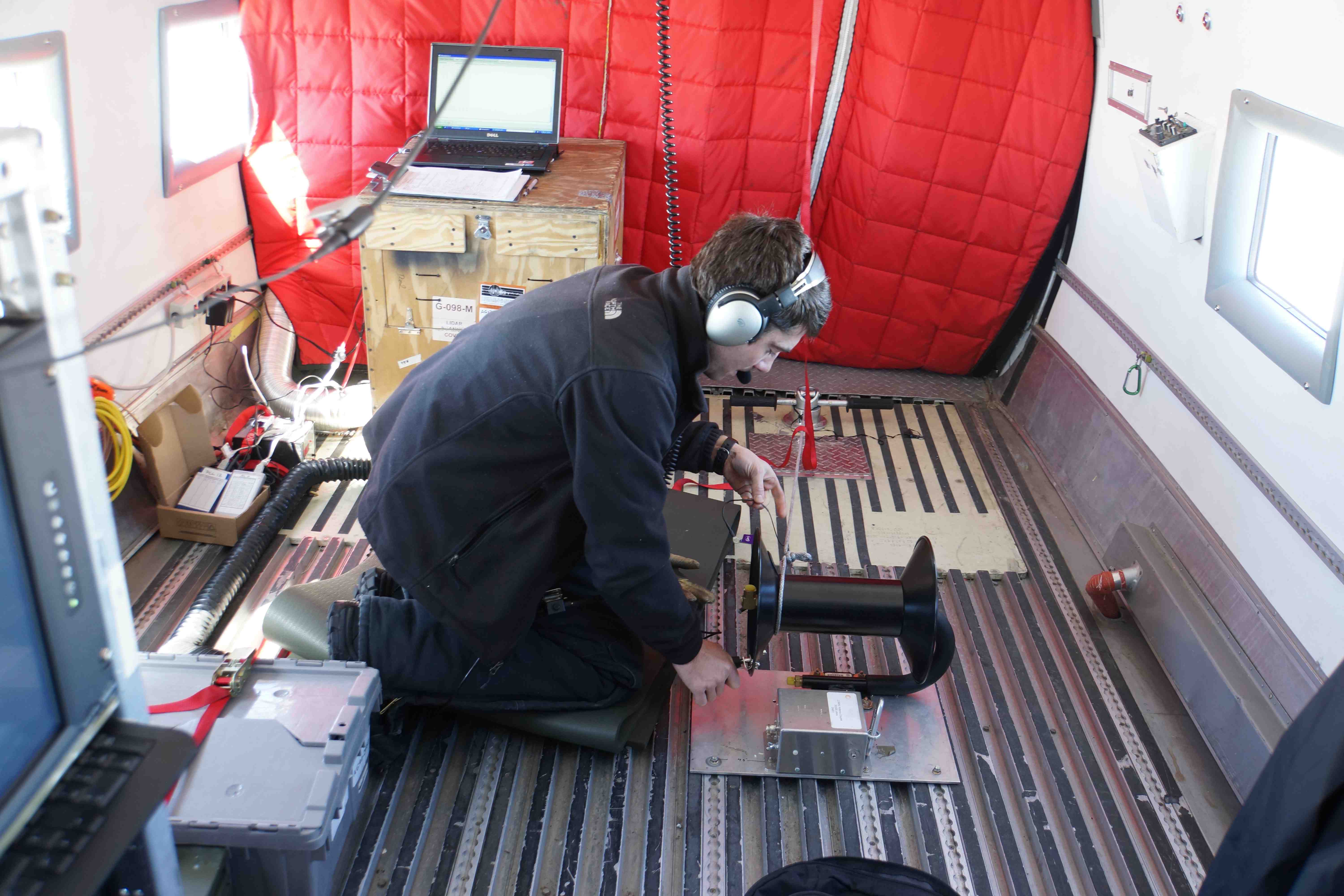
In addition to the 60MHz VHF radar, we also field a 2MHz HF radar. Rather than antennas under the wings, we unspool a ∼∼60m long wire antenna through a port in the floor. My attempts to get a clear picture of this antenna deployed while in flight have failed, so the best I have is one of Jamin preparing to reel the antenna back in.

The main factors determining how deep of a bed we can detect is the radar signal’s attenuation as it passes through the ice. Both warmer ice and saltier ice lead to higher losses, as does a rough surface that causes scattering. In some conditions, energy at 2MHz penetrates better than energy at 60MHz, at the cost of poorer vertical resultion due to the much longer wavelength.

We primarily fly this dual-frequency setup as a testbed for the REASON instrument that will be on the next mission to Europa.

Gravity

I’m continually amazed that we’re able to measure accelarations accurately enough to infer underwater topography based on local changes in gravitational acceleration. From a moving platform with turbulance, we’ll get precision on the order of a few mGal.¹⁷This requires integrating many measurements in order to get a usable signal to noise ratio, which means that we’re only able to detect features with a length scale of ~5km.¹⁸ The main complication when interpreting gravity data is that you’re actually measuring differences in density. If you assume less-dense sedimentary rocks underneath the water, you’re going to wind up balancing them out with a shallower water column, while if you assume denser rocks, you’ll infer deeper water.

Jamin Greenbaum recently published a paper¹⁹ improving the estimates of the cavity shape underneath the Totten Ice Shelf. His inferred geometry is shown below on the left.

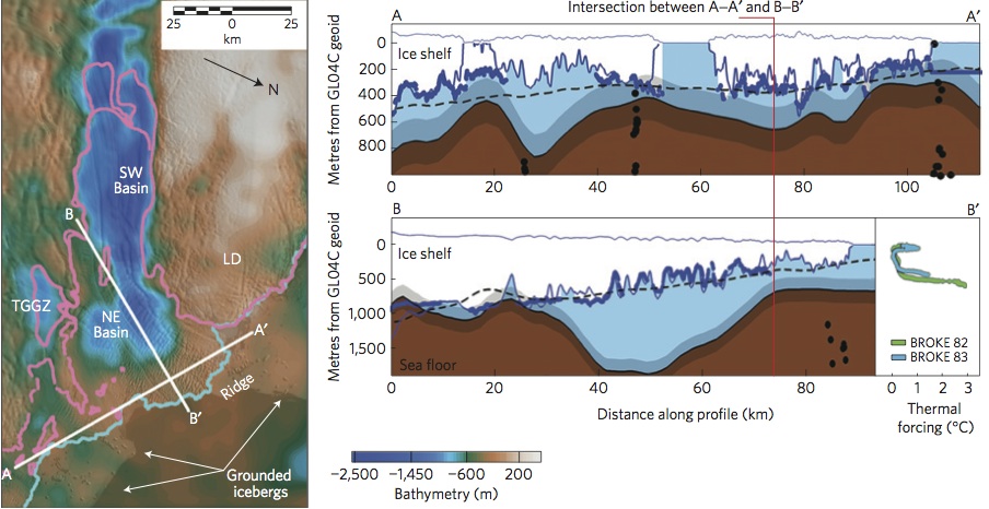
This was an important result because he showed that the ocean is deep enough that warm deep water is able to enter the cavity, which could explain why the glacier’s surface is lowering so quickly. It was also a significant improvement over the previous bathymetry – in the right plots of the above figure, you can see the old best-guess bathymetry as a dashed line.

Magnetics

We have two magnetometers on the plane. One is mounted inside near the cameras and and measures the 3 dimensional magnetic field vector. A much more precise one measuring only the magnitude is stuck way at the end of the tail boom, shown above. The idea behind this arrangement is that we want to understand how the airplane’s orientation and interaction with the earth’s magnetic field affects the measured field (you can see turns very clearly in the interior data), but we want the most accurate reading possible, taken as far away as possible from all the metal in the plane.

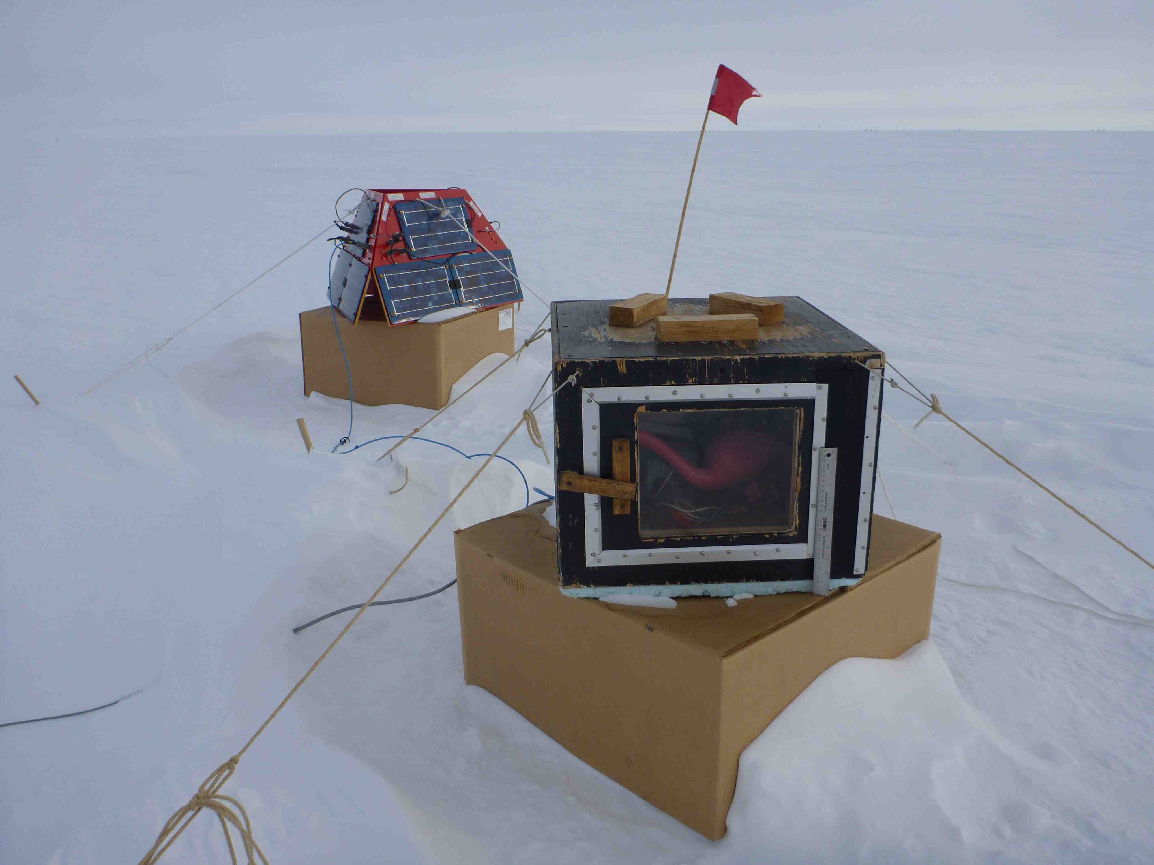
We also record the magnetic field at a base station. The above image shows the magnetometer housing and its solar charger. Data from this is used both to determine when to fly (it gets noisier at certain times of day) and used to correct the in-flight data to determine whether an anomaly is due to geological features or the earth’s magnetic field changing in response to solar activity. Any signal that’s different between the base and the airplane can be assumed to be from local topography, not the earth’s temporally varying magnetic field.

Igneous rocks tend to be magnetic, with their internal field aligned with what the earth’s field was when the rock formed, while ice and sedimentary rocks are not magnetic. This means that we can figure out what type of rocks are underneath the ice based on the magnetic signal that we observe! This process has been used to infer the presence of shallow volcanoes underneath the West Antarctic Ice Sheet. This matches very well with other observations indicating that the ice sheet is warmer and melting more than you’d expect for somewhere with globally average geothermal flux.

Determining the depth of the magnetic rocks can also be useful for interpreting gravity data. If something’s magnetic, you know that it’s denser than sediments would be, and anything that helps you constrain the density model will improve the gravity inversion. Depth can be inferred from the signal’s gradient – the deeper a feature is, the smoother the resulting signal will be.

Cameras

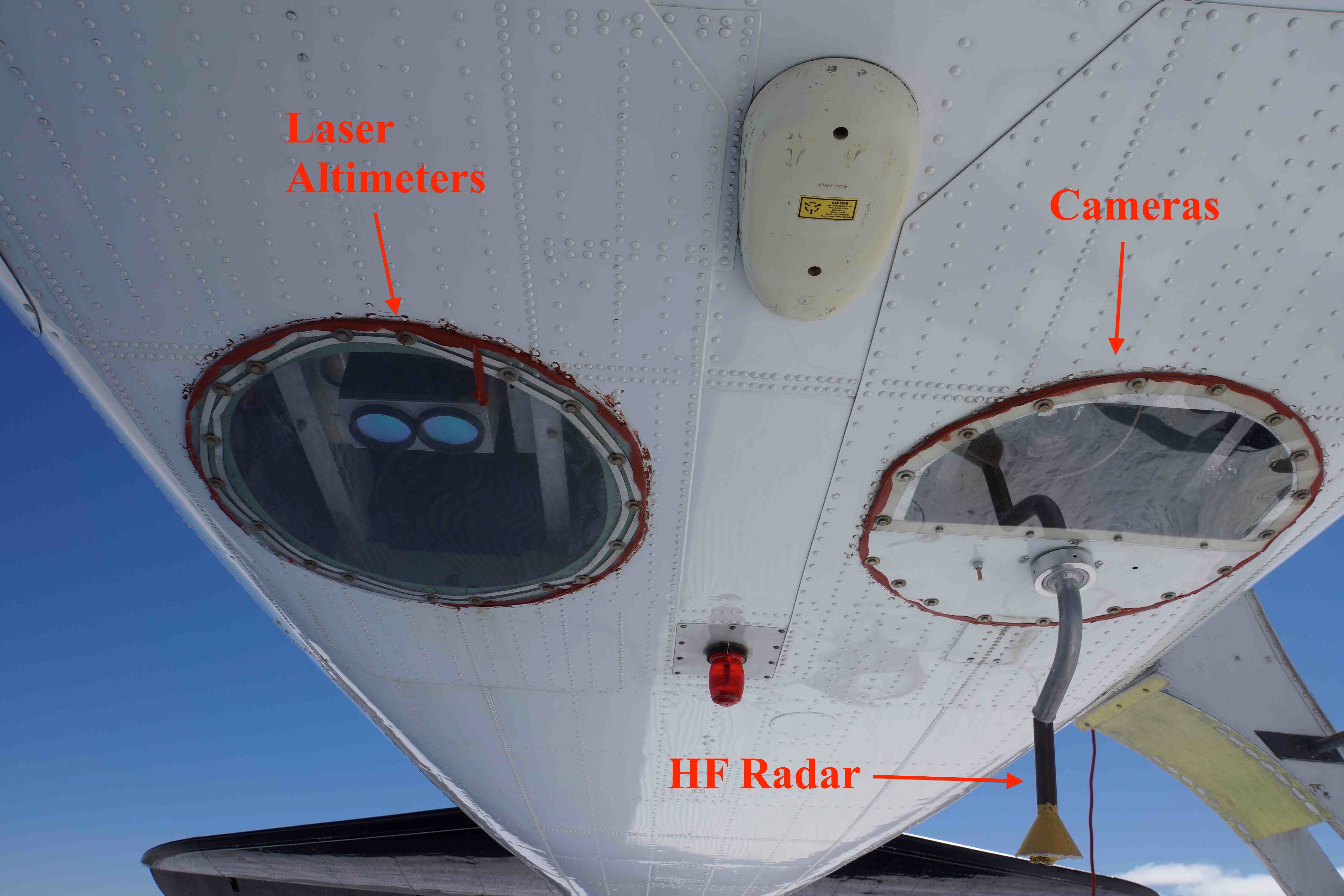
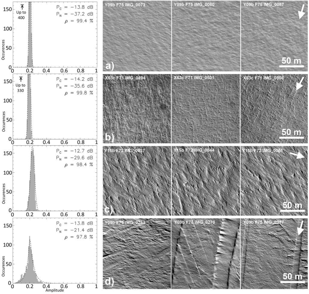
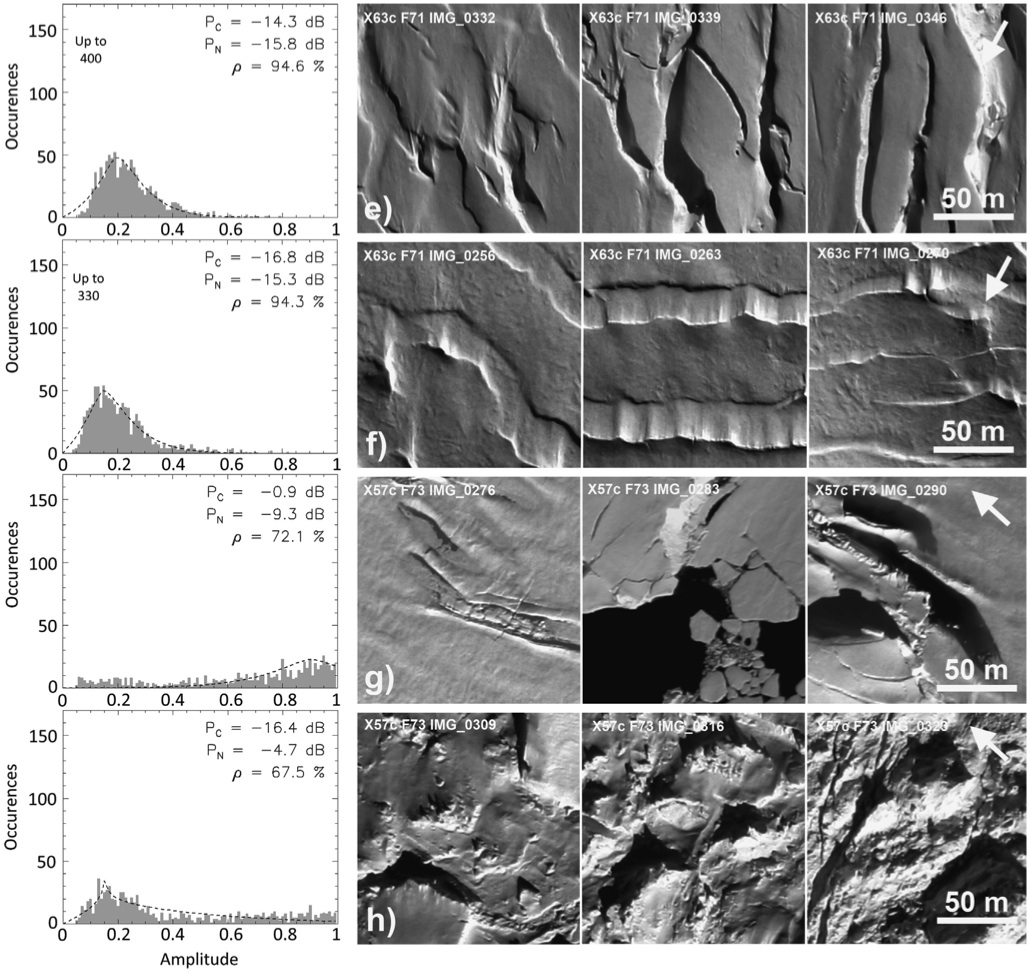
We don’t use camera data directly to answer any science questions,²⁰ but the pictures are useful for providing context for other data. This has included trying to figure out why we were missing laser data: Was it cloudy out? Were we in a heavily crevassed region? Were we over water? It has also been used to validate radar-derived surface roughness estimates. The below figure is from a paper by Cyril Grima²¹ and shows roughness parameters derived from a statistical examination of the returned radar pulse shape. The extracted parameters show an excellent qualitative agreement with the imagery.

Laser altimetry

We use lasers to very accurately measure the surface elevation of the ice sheet. Even where it is changing most rapidly, these changes are measured in meters per year, and our goal is to be able to detect changes of 5cm per year. From 2003-2009, ICESat collected laser altimetry from space, leading to a detailed map of where elevations are changing across Antarctica and Greenland.²²

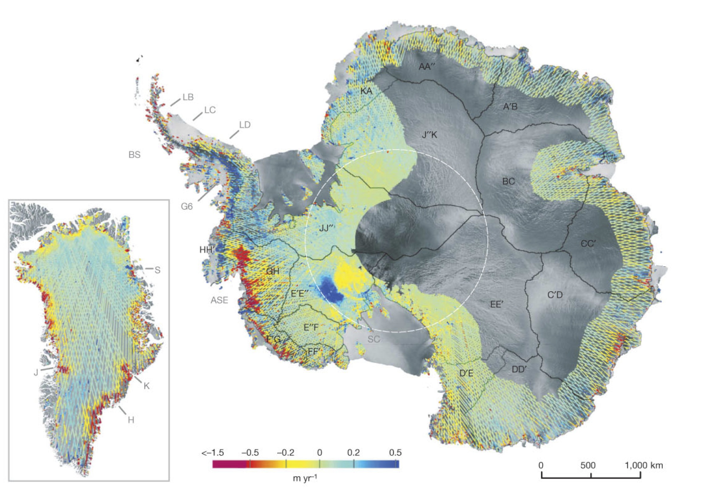
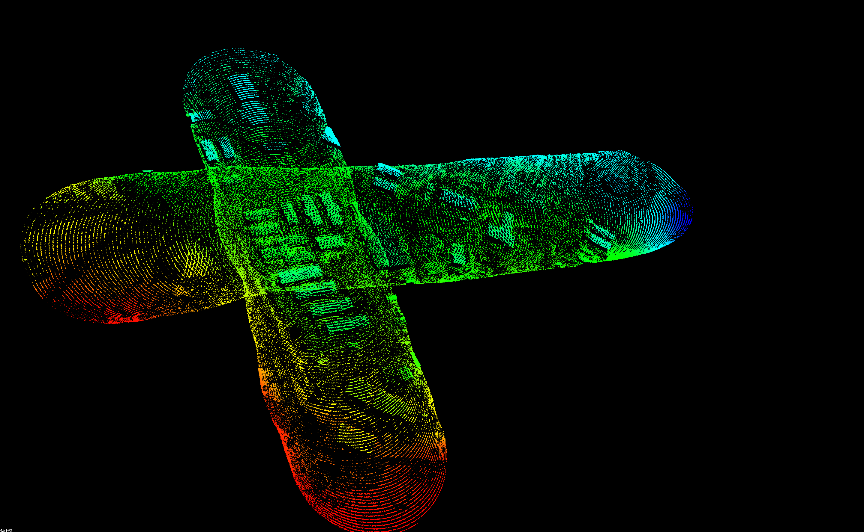
However, ICESat failed in 2009, and its replacement has not yet been launched. So, a number of groups (including ours) have been reflying ICESat tracks in an effort to extend the temporal record and hopefully connect it to ICESat II. Our system, ALAMO²³, includes an off-the-shelf single-beam Riegl altimeter, which is well characterized and used to determine the range to the surface. We also have a more temperamental scanning photon counting lidar that is a protopype of what will be on ICESat II. Its data points are dense enough to map individual buildings in McMurdo (below), but we mostly use its data to determine the ice’s surface slope, which is important when trying to compare two slightly offset repeat flights of the same line.

GPS, IMU

We have 4 GPS antennas mounted outside the plane: at the center, the tail, and on each wing. These are used to get absolute position in space. The IMUs measure accelations, and give us a very accurate orientation estimate – we have a little MEMs one mounted on rack 2, and a more precise one mounted directly to the PCL. After post-processing, we typically know our position to ∼∼2cm and our orientation to milli-radian accuracy.

While we don’t use this as science data in and of itself, knowing the airplane’s exact position is absolutely crucial for processing the other data. For example, the laser altimetry measurements are basically a 600m lever arm, and if we want to know the position of the end of that arm to centimeter accuracy, orientation matters.

Outside Air Temperature, Pressure

This is more metadata for our operation than science data. No major publications result from this, but I did use them to validate a correction for the speed of light in air, which primarily depends on pressure and temperature. I was utterly dumbfounded when I realized that the difference in conditions between the coast and inland domes could result in a 10cm bias in the altimetry data! We don’t consistently collect temperature and pressure data, but we always know our altitude. So, I needed to check that an altitude-based approximation to the speed of light would remove any geographical bias in our data.²⁴

1. KBA operates most of the non-military planes in Antarctica. ↩
2. BEDMAP2 was an effort to integrate all the available data into maps of Antarctica’s bedrock and ice thickness: Fretwell, P., Pritchard, H. D., Vaughan, D. G., Bamber, J. L., Barrand, N. E., Bell, R., Bianchi, C., Bingham, R. G., Blankenship, D. D., Casassa, G., and Others (2013). Bedmap2: improved ice bed, surface and thickness datasets for Antarctica. The Cryosphere, 7(1):375–393. ↩
3. There may still be such places, since I haven’t seen an updated map, but I was involved in a project that filled in the biggest hole. ↩
4. I’ll interchangeably refer to these airplanes as DC-3s and Baslers. DC-3 was the original designation; Basler is the name of a company that takes these old airplanes and entirely refurbishes them for Arctic/Antarctic work. ↩
5. JKB, the airplane shown in many off these photos, was used in WWII. ↩
6. Sadly, it would appear that this temperamental instrument is only collecting noise in this image. ↩
7. In addition to the DC-3s and Twin Otters, other groups have used LC-130s and P-3s to collect radar sounding data. They’re bigger, fly faster, and burn more fuel. ↩
8. This varies dramatically with elevation; we get significantly better than this flying over the Antarctic Plateau, and worse around the coast. ↩
9. If you’re at a coastal station, fuel is brought in on an ice breaker, and is less of a constraint. If you’re inland, that fuel is either brought in via a traverse (huge logistical operation) or flown in on LC-130s. Last season, at WAIS divide, the United States Antarctic Program used LC-130s to bring us fuel. They burn 3000 pounds of fuel an hour, and each delivery run from McMurdo provides enough fuel for ~3 of our survey flights. ↩
10. Endurance is primarily a function of how much fuel can be carried. The upper limit is neither the volume of the tanks nor the maximum weight that can get airborne – it’s the maximum weight that the airplane can safely land with, if an emergency landing were required just after takeoff. Nobody is going to be happy if you dump fuel over Antarctica. This means that each additional passenger costs ~15 minutes of extremely expensive survey time, and has been known to be a factor in deciding which additional instruments to install. Do you want the full suite of available instruments, or do you want an additional 30 minutes of survey time in order to reach that geologically interesting hole in the map? ↩
11. Pilots have legally- and contractually-mandated maximum duty day lengths, days off, maximum hours in the air per day, and rolling weekly/monthly flight hour maximums. ↩
12. This was … tough. The field camp was at an ice divide, meaning that weather systems could blow in from any of three directions, with very hard-to-predict timing. ↩
13. That was before GPS, so the positioning was only good to ~5km, and the radar data was recorded photographically, not digitally! The technology didn’t exist to digitize the received signals and write them to disk like we do now. ↩
14. Fretwell, P., Pritchard, H. D., Vaughan, D. G., Bamber, J. L., Barrand, N. E., Bell, R., Bianchi, C., Bingham, R. G., Blankenship, D. D., Casassa, G., and Others (2013). Bedmap2: improved ice bed, surface and thickness datasets for Antarctica. The Cryosphere, 7(1):375–393. ↩
15. NASA has produced some very fun visualizations of the improvement bewteen BEDMAP and BEDMAP2, as well as the ice surface / bed topography. We collected some of the data as a part of NASA’s Operation Ice Bridge (mostly in East Antarctica). link ↩
16. Of course, it was obsolete as soon as it came out, as everybody continues to collect more data. ↩
17. For context, the gravity field changes by ~300uGal/m as you get farther from the center of the earth, and 1G = 9.8m/s2 = 980Gal. Stationary instruments on the ground can measure to a precision of ~5uGal. ↩
18. For a fixed sampling rate, the slower you fly the better your data will be. We’re excited about the potential for mounting gravimeters on helicopters to get even higher-resolution data! Lower is also better, because you’re closer to the source. ↩
19. Greenbaum, J. S., Blankenship, D. D., Young, D. A., Richter, T. G., Aitken, A. R. A., Legresy, B., Schroeder, D. M., Roberts, J. L., Warner, R. C., van Ommen, T. D., and Siegert, M. J. (2015). Increased Ocean Access to Totten Glacier, East Antarctica. Nature Geos. ↩
20. We have recently learned that whale biologists are seriously interested in our data any time we fly over open water (which we do with some frequency for gravity data). It turns out that they’ve been fielding airplanes just to get the same type of imagery that we collect as a routine part of our operations. ↩
21. Grima, C., Schroeder, D. M., Blankenship, D. D., and Young, D. A. (2014a). Planetary landing-zone reconnaissance using ice-penetrating radar data: Concept validation in Antarctica. Planetary and Space Science. ↩
22. Pritchard, H. D., Arthern, R. J., Vaughan, D. G., and Edwards, L. A. (2009). Extensive dynamic thinning on the margins of the Greenland and Antarctic ice sheets. Nature, 461(7266):971– 975. /ref. ↩
23. Young, D. A., Lindzey, L. E., Blankenship, D. D., Greenbaum, J. S., de Gorordo, A. G., Kempf, S. D., Roberts, J. L., Warner, R. C., van Ommen, T., Siegert, M. J., and le Meur, E. (2014). Land-ice elevation changes from photon counting swath altimetry: First applications over the Antarctic ice sheet. Journal of Glaciology. ↩
24. I was impressed by my research group’s data management discipline when I was able to dig up and painlessly use 20+ year old data to do this analysis! ↩